
Chapter Eight
Ranking by Reordering Methods
The philosophy thus far in this book is depicted below in Figure 8.1. We start with input data about the items that we’d like to rank and then run an algorithm that produces a rating vector, which, in turn, produces a ranking vector. The focus has been on moving from left to right in Figure 8.1, i.e., transforming input data into a ranking vector. However, working backwards and instead turning the focus to the final product, the ranking vector itself, we are able to generate some new ideas, two of which appear in this chapter. These two new ranking methods follow the philosophy in Figure 8.2 below, which is to say, they completely bypass the rating vector.
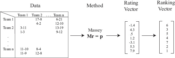
Figure 8.1 Philosophy of ranking methods of Chapters 4–7
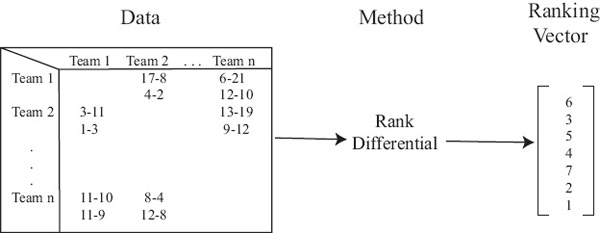
Figure 8.2 Philosophy of ranking methods of this chapter
Rank Differentials
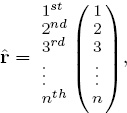
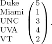
The most apparent feature of the ranking vector is that it is a permutation, which, as will soon become apparent, is the keyword for this chapter. Every ranking vector of length n is a permutation of the integers 1 through n that assigns a rank position to each item. For example, for our five team example, the Massey ranking vector is
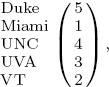
which assigns Duke to rank position 5, Miami to rank position 1, and so on. A ranking vector creates a linear ordering of the teams, yet it can also be used to consider pair-wise relationships. Pair-wise relationships are best portrayed with a matrix. Thus, the Massey ranking vector above creates the matrix of pair-wise relationships below. We call this matrix R since it contains information about rank differentials.
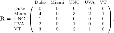
The 2 in the (UVA, Duke)-entry of R means that UVA is two rank positions above Duke in the Massey ranking vector. Thus, the entries in the matrix correspond to dominance.
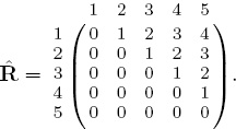
Each ranking vector of length n creates an n×n rank-differential matrix R, which is a symmetric reordering (i.e., a row and column permutation) of the following fundamental rank-differential matrix ![]() .
.
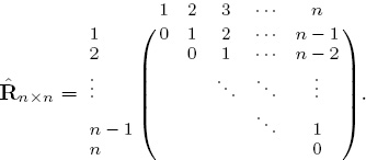
Notice the nice integer upper triangular structure of ![]() , which occurs because
, which occurs because ![]() is built from the associated fundamental ranking vector
is built from the associated fundamental ranking vector
in which the n items appear sorted in ascending order. In summary, there is a one-to-one mapping1 between a ranking vector and a rank-differential matrix. That is, every ranking vector r creates a rank-differential matrix R that can be expressed as R = QT![]() Q, where Q is a permutation matrix, and vice versa.
Q, where Q is a permutation matrix, and vice versa.
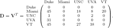
Because the fundamental rank-differential matrix is a team-by-team (or more generally an item-by-item) matrix, it is natural to compare it to other data matrices of the same size and type. For example, we can compare ![]() with the Markov voting matrix Vpointdiff of Chapter 6. This matrix contains the cumulative point differentials between pairs of teams. Point differentials, like rank differentials, contain information about the difference in the relative strength of two teams. However, the Markov voting matrices are created so that entries correspond to weakness. In order to relate Vpointdiff to dominance we simply compare R to the transpose of Vpointdiff. For clarity, for the remainder of this chapter, we talk about a general data differential matrix D. In most experiments, we use D =
with the Markov voting matrix Vpointdiff of Chapter 6. This matrix contains the cumulative point differentials between pairs of teams. Point differentials, like rank differentials, contain information about the difference in the relative strength of two teams. However, the Markov voting matrices are created so that entries correspond to weakness. In order to relate Vpointdiff to dominance we simply compare R to the transpose of Vpointdiff. For clarity, for the remainder of this chapter, we talk about a general data differential matrix D. In most experiments, we use D = ![]() .
.
We are now ready to cast the ranking problem as a reordering or nearest matrix problem. That is, given a data matrix D, which contains information about the past pair-wise comparisons of teams, find a symmetric reordering of D that minimizes the distance between the reordered data differential matrix and the fundamental rank-differential matrix ![]() . To be mathematically precise, given Dn×n, we want to find a permutation matrix Q such that ||QTDQ −
. To be mathematically precise, given Dn×n, we want to find a permutation matrix Q such that ||QTDQ − ![]() || is minimized. A permutation matrix Q applies a permutation of the integers 1 through n to the rows of the identity matrix. Thus, the optimization problem, which is defined over a permutation space, is constrained as follows.
|| is minimized. A permutation matrix Q applies a permutation of the integers 1 through n to the rows of the identity matrix. Thus, the optimization problem, which is defined over a permutation space, is constrained as follows.
The Running Example
We use the transpose of the point differential matrix as the data differential matrix D. Thus,
For a 5-team example, the fundamental rank-differential matrix
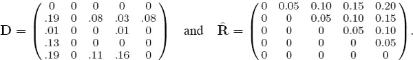
Our goal is to find the permutation of integers 1 through 5, and hence, the permutation of the five teams, that minimizes the error between the fundamental matrix ![]() and the reordered version of D. To deal with the varying scales, we first normalize each matrix by dividing by the sum of all elements. Thus the rounded normalized versions are
and the reordered version of D. To deal with the varying scales, we first normalize each matrix by dividing by the sum of all elements. Thus the rounded normalized versions are
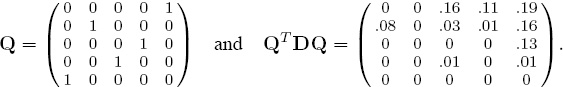
Even though n = 5 is small, there are still 5! = 120 different permutations to consider when reordering D. Using brute force (i.e., total enumeration), we discover that the permutation (5 2 4 3 1) is optimal, which creates the permutation matrix Q and, which, in turn, creates the reordered data differential matrix QTDQ shown below.
The reordered matrix QTDQ is closest to the fundamental rank-differential matrix ![]() . Figure 8.3 uses MATLAB’s cityplot view to show a side-by-side comparison of the reordered normalized D and normalized
. Figure 8.3 uses MATLAB’s cityplot view to show a side-by-side comparison of the reordered normalized D and normalized ![]() matrices below.
matrices below.
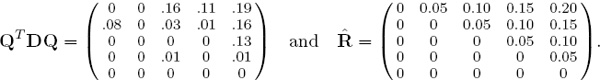
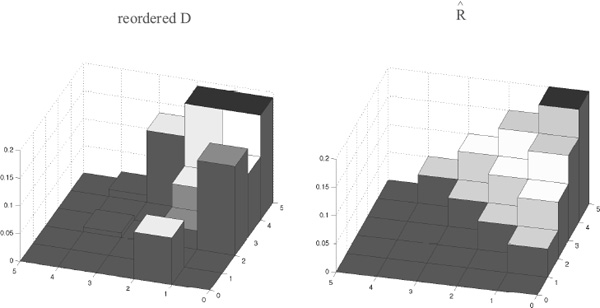
Figure 8.3 Cityplot of reordered D (i.e., Q![]() Q) and
Q) and ![]() and for the 5-team example
and for the 5-team example
Reordering the five teams from the original ordering of (1 2 3 4 5) to the optimal ordering of (5 2 4 3 1) produces a data differential matrix that is closest to the stair-step form of the fundamental rank-differential matrix ![]() .
.
In summary, the method of rank differentials is unlike previously discussed ranking methods. In particular, it searches for the nearest rank-differential matrix to a given data matrix. And since each rank-differential matrix corresponds to a ranking, it is yet another ranking method to add to our arsenal.
The Q*bert Matrix
It’s time to give credit where credit is due and in this case the credit goes to David Gottlieb, the inventor of the popular 1982 arcade game called Q*bert. Figure 8.4 shows the unmistakable similarities between the cityplot of fundamental rank-differential matrix ![]() and the Q*bert game board. In honor of Gottlieb’s game, we sometimes refer to
and the Q*bert game board. In honor of Gottlieb’s game, we sometimes refer to ![]() , the fundamental rank-differential matrix, by the shorter and more memory-friendly name of the Q-bert matrix.
, the fundamental rank-differential matrix, by the shorter and more memory-friendly name of the Q-bert matrix.
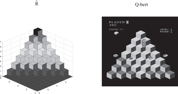
Figure 8.4 Fundamental rank-differential matrix ![]() and the Q*bert game board
and the Q*bert game board
Solving the Optimization Problem
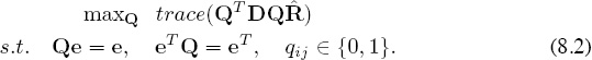
Let’s examine the optimization problem of Expression (8.2). The goal is to find a symmetric permutation of D that minimizes the difference between the permuted data matrix QTDQ and the fundamental rank-differential matrix ![]() . For an n-item list, there are n! possible permutations to consider. This, of course, means the brute force method of total enumeration that we used in the previous section is not practical. Case in point: for the tiny five-team example, to find the optimal permutation we had to check 5! = 120 permutations. Doubling the number of teams requires consideration of 10! = 3, 628, 800 permutations. Fortunately, with some clever analysis, we can avoid considering all n! permutations.
. For an n-item list, there are n! possible permutations to consider. This, of course, means the brute force method of total enumeration that we used in the previous section is not practical. Case in point: for the tiny five-team example, to find the optimal permutation we had to check 5! = 120 permutations. Doubling the number of teams requires consideration of 10! = 3, 628, 800 permutations. Fortunately, with some clever analysis, we can avoid considering all n! permutations.
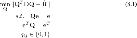
The matrix formulation of the optimization problem below reveals its classification as a binary integer nonlinear program.
minQ ||QTDQ − ![]() ||
||
s.t. Qe = e, eTQ = eT, qij ∈ {0, 1}
The matrix norm in the objective function affects the type of nonlinearity. For example, if the norm is of the Frobenius type, this nonlinearity is quadratic. While quadratic integer programs are challenging, there are some properties of the Frobenius norm and the Q-bert matrix ![]() that can be exploited to significantly reduce computation. For instance, with some algebra
that can be exploited to significantly reduce computation. For instance, with some algebra
![]()
Since trace(DTD) and trace(![]() T
T![]() ) are constants, this means that the original minimization problem is equivalent to the maximization problem below.
) are constants, this means that the original minimization problem is equivalent to the maximization problem below.
The change in the objective function brings significant computational advantages. All optimization algorithms require the computation of the objective function repeatedly and this computation is typically the most expensive step in an iterative algorithm. Fortunately, the equivalent expression of Equation (8.2) is especially efficient due to the known structure of ![]() . Even more advantageous is the fact that
. Even more advantageous is the fact that ![]() need not be formed explicitly. In fact, the pseudocode below shows how the computation of the Frobenius objective function can be coded very efficiently.
need not be formed explicitly. In fact, the pseudocode below shows how the computation of the Frobenius objective function can be coded very efficiently.
Pseudocode to compute trace(QTDQ![]() ) efficiently
) efficiently
  function [f]=trQtDQR(D,q);
  INPUT: D = data matrix of size n × n
          q = permutation vector of size n × 1
  OUTPUT: f = trace(QTDQ)
  n=size(D,1);
  [sortedq,index]=sort(q);
  clear sortedq;
  f=0;
  for i=2:n
       for j=1:i−1
            f=f+(i−j)*D(index(i),index(j));
       end
  end
The Relaxed Problem
The Frobenius formulation of the Q-bert problem gave it two tags, the quadratic tag and the integer tag. Of these two, the integer tag is more challenging. Often times, integer programs are solved approximately by the technique of relaxation, which relaxes the nasty integer constraints into continuous constraints. Thus, the relaxed Q-bert problem is given by the quadratic program below.
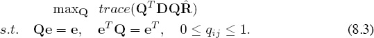
As a result, Q is no longer a permutation matrix, but instead is a doubly stochastic matrix (i.e., a matrix whose rows and columns sum to 1). Thus, rather than optimizing over a permutation space, we optimize over the set of doubly stochastic matrices. Sometimes, the optimal solution to the relaxed problem is integer, in which case it is also optimal for the original quadratic integer program. In this case, the extreme points of the relaxed constraint set are points in the original constraint set. Unfortunately though, the quadratic nature of the objective function allows for optimal solutions to occur in the interior of the feasible region, in which case, an optimal solution for the relaxed problem would not be feasible for the original problem. Often times the noninteger solution of the relaxed problem can be rounded to the nearest integer solution, creating a feasible solution to the original problem. Unfortunately in this case, there is no obvious rounding strategy that will guarantee that the rounded solution is anywhere near optimal for the original problem. In fact, you’ve really got another quadratic integer program on your hands. That is, find the nearest permutation matrix to the given doubly stochastic matrix. In summary, in our case, relaxation is disappointing.
An Evolutionary Approach
While relaxing the quadratic integer program is not promising, fortunately, another optimization approach is. Rather than trying to find a permutation matrix Q, we can equivalently try to find a permutation vector q that can be used to reorder the data differential matrix D. The reordering formulation tries to find the permutation q of integers 1 through n such that D(q, q) is closest to ![]() in the sense that
in the sense that
![]()
where q ∈ pn means that q must belong to the set of all n × 1 permutation vectors. For example, the permutation vector q = ![]() symmetrically reorders2
symmetrically reorders2
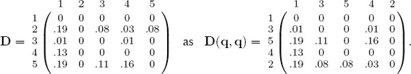
Notice that the elements of D are simply relocated in D(q, q).
Matrix reorderings have been well-studied and have a rich history of uses from pre-conditioners for linear systems to preprocessors for clustering algorithms [9, 66, 7]. Thinking of the problem as a matrix reordering problem does not reduce the search space. There are still n! possible permutations that reorder D, yet optimization problems involving permutations are often tractable through a technique known as evolutionary optimization.
Evolutionary optimization, as the name suggests, takes its modus operandi from natural evolution. The idea is to start with some initial population of p possible solutions, which in this case, are permutations of the integers 1 through n. Each member of the population is evaluated for its fitness. In this case, the fitness of a solution x is ||D(x, x) − ![]() ||. The fittest members of the population are mated to create children that contain the best properties of their parents. Continuing with the evolutionary analogies, the less fit members are mutated in asexual fashion while the least fit members are dropped and replaced with immigrants. This new population of p permutations is evaluated for its fitness and the process continues. As the iterations proceed, it is fascinating to watch Darwin’s principle of survival of the fittest. The populations march toward more evolved, fitter collections of permutations. Perhaps more fascinating is the fact that there are theorems proving that evolutionary algorithms converge to optimal solutions in many cases and near optimal solutions under certain conditions [55]. Unfortunately, evolutionary algorithms are often slow-converging, which explains their application to problems that are known as either very challenging or nearly intractable. For instance, evolutionary algorithms gained notoriety for their ability to solve larger and larger traveling salesman problems, the famously intractable problem described in the Aside on p. 104.
||. The fittest members of the population are mated to create children that contain the best properties of their parents. Continuing with the evolutionary analogies, the less fit members are mutated in asexual fashion while the least fit members are dropped and replaced with immigrants. This new population of p permutations is evaluated for its fitness and the process continues. As the iterations proceed, it is fascinating to watch Darwin’s principle of survival of the fittest. The populations march toward more evolved, fitter collections of permutations. Perhaps more fascinating is the fact that there are theorems proving that evolutionary algorithms converge to optimal solutions in many cases and near optimal solutions under certain conditions [55]. Unfortunately, evolutionary algorithms are often slow-converging, which explains their application to problems that are known as either very challenging or nearly intractable. For instance, evolutionary algorithms gained notoriety for their ability to solve larger and larger traveling salesman problems, the famously intractable problem described in the Aside on p. 104.
Figure 8.5 below is a pictorial representation of the main ideas behind evolutionary algorithms, particularly when applied to the ranking problem. This wonderful global view of the algorithm is thanks to College of Charleston graduate Kathryn Pedings. Kathryn used this figure in a few talks and as part of a poster [18]. She is a lively and interesting speaker, so it is unfortunate that readers can’t hear Kathryn describing her work in person. As a paltry substitute, we have attempted to simulate Kathryn’s explanation of Figure 8.5 by attaching text labels to her original figure. Simply follow the annotations in numerical order.
ASIDE: The Traveling Salesman Problem
The Traveling Salesman Problem (TSP) refers to the problem of planning a tour for a salesman who needs to visit n cities, once each. Certain variants of the problem require the salesman to start and end at the same city, presumably his hometown. The goal is to choose the minimum cost route where cost can be defined in various ways, such as total time or distance traveled. Each possible route can be considered a permutation of the n cities. Advanced variants of the TSP add constraints. For example, the salesman cannot travel more than 500 miles in a day, visit two consecutive cities in the same state, etc. Despite the elegantly simple statement of the problem, the TSP is famously hard (in fact, NP-hard, for those familiar with the term) to solve due to something called state space explosion. In its standard unconstrained formulation, the TSP has n!/2 possible routes that must be considered. The function n! explodes quickly even when n grows slowly. See Table 8.1. In the pre-computer era, heuristic algorithms were implemented to approximate the optimal solution. A TSP with n = 10 cities was considered large in those days. With computers, research on TSPs took off and, in turn, so did their use.
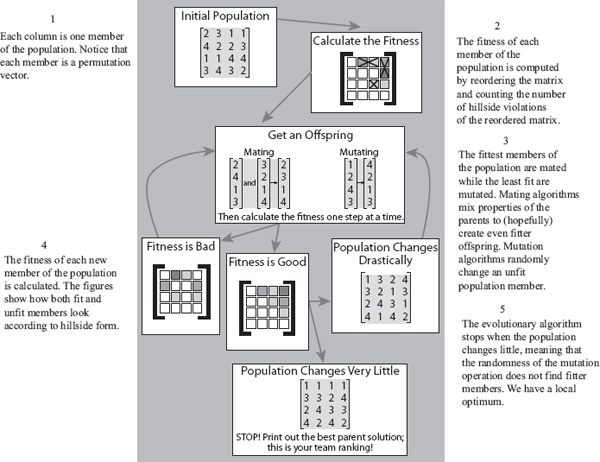
Figure 8.5 Overview of steps of evolutionary algorithm for ranking problem
Recently, evolutionary algorithms have led the way in TSP research. The size of TSPs that can be solved are now on the order of tens of thousands of cities. In fact, in 2006 a TSP with n = 85,900 cities was solved. As a result of the increase in the size of solvable TSPs, they have seen more widespread use. Today airlines use TSPs to schedule flight routes and computer hardware companies use TSPs to place copper wiring routes on circuit boards.
Advanced Rank-Differential Models
Most of the ranking methods that have been presented so far in this book allow for consideration of multiple statistics in their creation of a ranking. So too does the rank-differential method. The k multiple statistics can be combined into a single data matrix D = α1D1 + α2D2 + · · · + αkDk with each differential matrix Di given a scalar weight αi. Then the same optimization problem, minq∈pn ||D(q, q) − ![]() || is solved. Or the k differential matrices can be treated separately in the optimization as
|| is solved. Or the k differential matrices can be treated separately in the optimization as
![]()
Again, we recommend using an evolutionary algorithm to solve the optimization problem. Notice that the second formulation is much more expensive since calculating the fitness of each population member at each iteration requires k matrix norm computations.
Table 8.1 Explosion of n! function
n |
n! |
5 |
120 |
10 |
≈ 3.6 × 10⁶ |
25 |
≈ 1.6 × 1025 |
50 |
≈ 3.0 × 1064 |
100 |
≈ 9.3 × 10157 |
Summary of the Rank-Differential Method
The Notation
D is the item-by-item data matrix containing pair-wise relationships such as differentials of points, yardage or other statistics.
![]() is the fundamental rank-differential matrix.
is the fundamental rank-differential matrix.
Q is a permutation matrix.
q is the permutation vector corresponding to Q.
D(q, q) is the reordered data-differential matrix QTDQ.
The Algorithm
1. Solve the optimization problem
![]()
where pn is the set of all possible n×1 permutation vectors. We recommend using an evolutionary algorithm.
2. Use the optimal solution q of the above problem to find the ranking vector by sorting q in ascending order and storing the sorted indices as the ranking vector.
Properties of the Rank-Differential Method
• All the ranking methods discussed thus far produce both a rating and a ranking vector. The rank-differential method is the first to produce just a ranking vector.
• This method finds a reordering of the data differential matrix D that is closest to the fundamental rank-differential matrix ![]() . While closeness can be measured in many ways, it was demonstrated on page 102 that the Frobenius measure is particularly efficient.
. While closeness can be measured in many ways, it was demonstrated on page 102 that the Frobenius measure is particularly efficient.
• Because the optimization problem is very challenging (in fact, NP-hard), the rank-differential method is slower and more expensive than the other ranking methods presented in this book. Thus, it may be limited to smaller collections of items. For example, ranking sports teams is within in the scope of the method, but, unless clever implementations are discovered, ranking webpages on the full Web is not.
• Any data matrix can be used as input to the rank-differential matrix. In this chapter, we recommended using the point differential matrix of the Markov method, however, any differential data could be used.
ASIDE: The Rank-Differential Method and Graph Isomorphisms
The rank-differential method is intimately related to the graph and subgraph isomorphism problems.3 In such cases, D and ![]() represent the (possibly weighted) adjacency matrices of two distinct graphs. The goal is to determine if one graph can have its nodes relabeled to produce the other. If it can, then ||QTDQ −
represent the (possibly weighted) adjacency matrices of two distinct graphs. The goal is to determine if one graph can have its nodes relabeled to produce the other. If it can, then ||QTDQ − ![]() || = 0 and the two graphs are said to be isomorphic. If it cannot, then ||QTDQ −
|| = 0 and the two graphs are said to be isomorphic. If it cannot, then ||QTDQ − ![]() || is minimized to produce a relabeling of D’s nodes that brings D closest to
|| is minimized to produce a relabeling of D’s nodes that brings D closest to ![]() . Our formulation is different on two counts. First, our formulation is a bit more general in that D and
. Our formulation is different on two counts. First, our formulation is a bit more general in that D and ![]() do not have to represent adjacency matrices. Second, our formulation, on the other hand, is a bit more specific because
do not have to represent adjacency matrices. Second, our formulation, on the other hand, is a bit more specific because ![]() has its very special structure. Graph isomorphisms have been used successfully in a variety of applications ranging from the identification of chemical compounds to design of electronic circuit boards. Progress that we make here can be applied there, emphasizing the value of the connection between our problem and the graph isomorphism problem.
has its very special structure. Graph isomorphisms have been used successfully in a variety of applications ranging from the identification of chemical compounds to design of electronic circuit boards. Progress that we make here can be applied there, emphasizing the value of the connection between our problem and the graph isomorphism problem.
Rating Differentials
The ranking methods of Chapters 4–7 each produce a rating vector that is then sorted to give a ranking vector. The rank-differential method of the previous section is the first to bypass the rating vector altogether and produce only a ranking vector. Though the name uses the word rating, the same is true of the rating-differential method presented in this section. It skips the rating vector and goes directly to the ranking vector. Nevertheless, we will see that the word rating in the method’s name is appropriate.
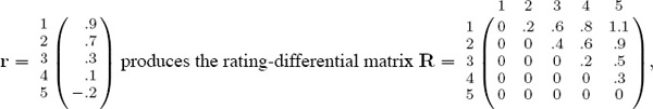
Consider the Massey rating vector r for the five team example,
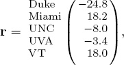
which creates the following rating-differential matrix
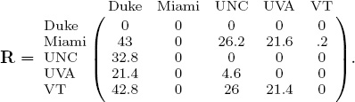
We’ve admittedly used the same notation for both differential matrices, though this should cause no confusion. The entries in the matrix indicate the type of differential matrix. A rank-differential matrix contains only integers, while a rating-differential matrix has scalars. Unlike the rank-differential setting, where there is a single fundamental rank-differential matrix, there is no single fundamental rating-differential matrix. Yet there is a fundamental structure. Consider a rating vector that is already in the correct sorted order. For example, the rating vector
which has a very characteristic structure. Every rating-differential matrix R can be reordered to have this structure.
A rating-differential matrix R is in fundamental form if
rij = 0, ∀ i ≥ j (strictly upper triangular)
rij ≤ rik, ∀ i ∋ j ≤ k (ascending order across rows)
rij ≥ rkj, ∀ j ∋ i ≤ k (descending order down columns).
The cityplot of R(q, q) resembles a hillside. See Figure 8.6. Thus, we sometimes refer to the fundamental form as the hillside form.4 Every rating vector creates a rating-differential matrix that can be reordered to be in fundamental form. The ordering of the items required to produce the reordering is a permutation of the integers 1 through n. And this permutation is precisely the ranking vector.
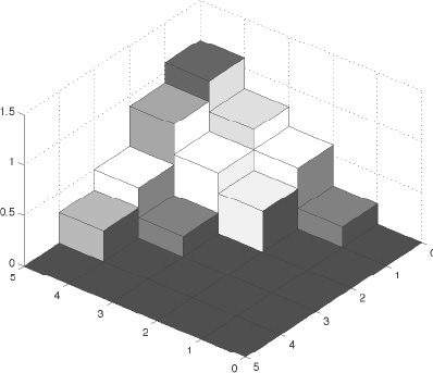
Figure 8.6 Cityplot of rating-differential matrix R in fundamental or hillside form
Astute readers are probably questioning us now: didn’t the above logic produce a ranking vector by assuming the availability of a rating vector? How valuable is that? If we had a rating vector, then of course we have a ranking vector. The example in the next section shows how the definitions produced by this seemingly backward logic lead to a new, viable ranking method that does not require the presence of a rating vector first.
The Running Example
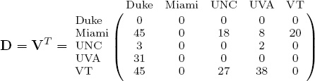
The rating-differential method begins with a team-by-team data matrix as input. For the same reason mentioned in the rank-differential section, it makes sense to use a matrix of differential data D. In this example, we use the transpose of the Markov voting matrix V of point differentials, denoted VT, since here it makes sense to think of votes as an indicator of strength rather than weakness. The goal of the rating-differential method is to find a reordering of D that brings it to the fundamental form of the box on page 108 or as near to that form as possible. For the five team example,
and there are 5! permutations of the five teams that will symmetrically reorder the matrix. Using the brute force method of total enumeration we find that the permutation
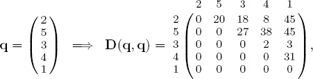
which, though not in fundamental form, is closest with the fewest constraint violations (just six). Sorting the optimal permutation vector q and keeping track of the indices produces the ranking vector
Solving the Reordering Problem
The rating-differential problem can be stated as: find the permutation q such that the reordered data differential matrix D(q, q) violates the minimum number of constraints of the box on page 108. For a collection of n items, there are n! possible permutations. The enormous state space and the presence of permutations make evolutionary optimization an attractive and appropriate methodology. Because the rank differential and rating-differential problems are so closely related, the population, mating, and mutating operations are identical. Only the fitness function must be changed for the rating-differential problem. In this case, the fitness of a permutation, which is a member of the population, is given by the number of constraints of the box on p. 108 that are violated.
While the evolutionary approach to solving the rating-differential problem can be used, the best technique is to transform the problem into a binary integer linear program (BILP) that can then be relaxed into a linear program (LP). Rather than describing this method here, we postpone that discussion until Chapter 15 as it can be shown that the rating-differential method is actually a special case of the rank-aggregation method described in that chapter. The rating-differential problem is revisited on page 194.
ASIDE: More College Basketball
The rating-differential method formed a large part of the M.S. thesis of College of Charleston graduate student Kathryn Pedings. As most graduate students do, Kathryn gave talks and posters describing her work at various conferences and universities. The most distant of these took place at Tsukuba University about an hour outside of Tokyo, Japan, where she used the following figures to illustrate her work. The figure below shows two point differential matrices for the eleven teams in the 2007 Southern Conference of men’s college basketball.
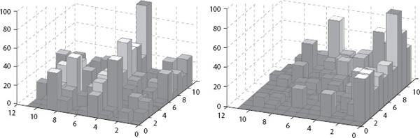
The cityplot on the left shows the matrix in its original ordering, where no structure is apparent. The cityplot on the right is the same matrix reordered according to the rating-differential method, where the hillside structure is revealed. Then in the following table she compared the rating-differential rankings (which she referred to as evolutionary optimization) with the Massey and Colley rankings.
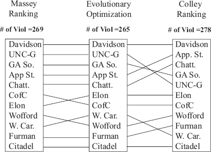
Notice that the rating-differential method of this section was the ranking with the fewest hillside violations. If this is a priority, then clearly the rating-differential method is the method of choice as it is guaranteed to produce a ranking with the fewest hillside violations.
Summary of the Rating-Differential Method
—Labeling Conventions
D is the item-by-item data matrix containing pair-wise relationships such as differentials of points, yardage, or other statistics.
q is the permutation vector that defines the reordering of D.
—The Algorithm
1. Solve the optimization problem
![]() (# of constraints listed on page 108 that D(q, q) violates)
(# of constraints listed on page 108 that D(q, q) violates)
While an evolutionary algorithm works, we recommend using the Iterative LP method described later in Chapter 15.
2. The optimal solution q of the above problem is used to find the ranking vector; sort q in ascending order and store the sorted indices as the ranking vector.
—Attributes
• The ranking methods discussed in previous chapters of this book produce both a rating and a ranking vector. The rank-differential and the rating-differential methods both produce a ranking vector only.
• The rating-differential method finds a symmetric reordering q of the differential matrix D that brings D(q, q) as close to hillside form as possible.
• Because the optimization problem is challenging (in fact, NP-hard), the rating-differential method is slower and more expensive than the other ranking methods presented in this book. Thus, it may be limited to smaller collections of items. For example, ranking sports teams is within in the scope of the method, but ranking webpages on the full Web is not. Yet despite being limited to smaller collections, the rating-differential method is a totally new approach to ranking.
• Any data matrix can be used as input to the rating-differential method. In this chapter, we recommended using a point differential matrix, however, other data differential matrices would work as well.
• Like the rank-differential method, the rating-differential method seems to work particularly well for collections of items that have many direct pair-wise relationships. That is, collections for which the item-by-item matrix has many connections. Consequently, the rating-differential method may perform poorly on a collection of items with few connections.
By The Numbers —
18 = number of players that were killed in football games in 1904.
— This and the countless broken bones, fractured sculls, broken necks, wrenched legs, and many other gruesome injuries caused Theodore Roosevelt to threaten to outlaw college football in 1905.
— The Big Scrum, by John J. Miller
1The mapping is one-to-one if no ties occur in the ranking vector. See Chapter 11 for a full discussion of ties.
2A symmetric reordering uses the same permutation to reorder both the row and the column indices.
3We thank Schmuel Friedland for pointing out this connection.
4Actually, we sometimes call this the R-bert form. Arcade fans might remember the 1982 game Q-bert in which a character of the same name hops around on a stair-step hillside that, with its equally spaced stairs, looks just like ![]() , the fundamental rank-differential matrix of Figure 8.3. Because the rating-differential matrix has unequally spaced stairs, we jokingly call this the R-bert, rather than the Q-bert, form.
, the fundamental rank-differential matrix of Figure 8.3. Because the rating-differential matrix has unequally spaced stairs, we jokingly call this the R-bert, rather than the Q-bert, form.