Chapter Nine

Point Spreads

Something would be amiss in a book about ratings and rankings if there was not a discussion of point spreads because beating the spread is the Holy Grail for those in the betting world. However, the goals and objectives of scientific ratings systems are not generally in line with those of bookmakers or gamblers.

A good scientific rating system tries to accurately reflect relative differences in the overall strength of each team or competitor after a reasonable amount of competition has occurred. Perhaps the most basic goal is to provide reasonable rankings that agree with expert consensus and reflect long-term ability for winning. Most of the popular scientific systems are moderately successful at producing ratings that are consistent with win percentages. But, as illustrated in the discussion of the Keener ratings on page 49, there is a big gap between estimating win percentages and estimating point spreads, and just because a system does a reasonably good job at the former is no indication of its ability to provide information concerning the latter.

An ultimate target for some is to design a system for which relative differences in the ratings that their system produces somehow leads to accurate predictions of scoring differences when two teams meet. While this is generally an impossible goal, it nevertheless continues to occupy the attention of rating system developers—after all, even Isaac Newton never lost his passion for alchemy. However, even if you achieve the rater’s equivalent of turning lead into gold, it is not axiomatic that this will translate into “sure bets” because your bookmaker or casino has a different concept of “point spread.”

What It Is (and Isn’t)

Many novices fail to understand the true meaning of “the point spread” and the mechanisms used to construct the “spread” for a given game. The point spread put forth by bookmakers is in no way meant to be an accurate reflection or prediction of how much better one team is than another, and making accurate predictions of scoring differences is nowhere near the aim of bookies. In some sense they have an easier task. The entire purpose of the point spread that is published by a bookmaker for a given game is to attract an equal amount of money that is bet on both teams. Doing so ensures two things.

1. It helps to maximize the betting activity.

2. It balances the amount the bookie takes in against the amount he must pay out.

To understand how these two features contribute to the bookmaker’s profit, you need to know exactly how a bookie makes money.

The Vig (or Juice)

The bookmaker generally does not make money by betting against you and having you lose. Good bookies don’t care whether you win or lose your bet because their profit is usually derived from the vig, short for vigorish¹ (or juice, as it is sometimes called) that is simply a fee or commission that you are charged for the bookmaker’s service. When the bookmaker is successful at attracting an equal amount of money that is bet on each team in a given game, then, regardless of who wins, the bookie’s net pay out is zero, and his vig becomes pure profit.

Why Not Just Offer Odds?

If the bookmaker did not issue a spread but rather only took bets on which team will win a given game, then in order to maintain a balance of what is taken in against what is payed out, the payoff on a winning bet would have to be tied to the odds in favor of winning. Consequently, when a strong team is matched against a substantially weaker team, a gambler who wants to bet on the strong team is forced to risk a relatively large amount in order to win just a small amount. Furthermore, most savvy gamblers won’t make a “win bet” on a likely loser even if the odds are enticing. In other words, offering only odds will usually result in decreased betting activity, and this is bad for the bookie because the total vig is directly tied to the number of bets being placed.

Somewhere around the mid 1930s Charles K. McNeil² realized that by offering gamblers the opportunity to bet against a published spread, bookies were able to attract more action (and thus generate more vig) than would be realized by only offering odds in favor of winning. Gambling had recently become legal in Nevada in 1931, and as soon Las Vegas bookmakers became aware of McNeil’s new idea, they realized its advantage and immediately adopted it. Ever since, spread betting has been the standard mechanism for sports wagering.

How Spread Betting Works

As we have said, the bookmaker’s purpose is to simultaneously maximize and balance the activity on both sides of any wager that he wants to make. He offers a point spread to create a handicap against the favored team so that instead of simply betting on the event that team i will beat team j, the wager is on the event that team i will beat team j by more (or less) than the offered spread. The bookmaker’s job is to determine the point spread that will generate an equal amount of action on each side of this wager.

On the surface it may seem as though the spread should be calculated to offer each side an equal probability of winning. However, the money bet on an event is rarely equally distributed even if the wager is “fair,” so spreads are revised as game time nears. Bookmaking is a black art not meant for the faint of heart, and successful bookies need to be more than numbers and stats people—they also need to be pretty good psychologists and students of human nature who have an excellent understanding of their clientele.

Beating the Spread

Just exactly what does the phrase “beating the spread” mean? Well, it can happen in two ways. If you a bet on a team and that team wins by more than the advertised point spread, then you win—you “beat the spread!” But there is another way you can do it. If you bet on the team that is not favored, and if they win, then so do you. But if they lose by fewer points than the published spread, then you still win—so again, you “beat the spread!” Let’s look at a couple of examples.

Suppose that your bookmaker has listed the BRONCOS to beat the CHARGERS by 7 points, and suppose that the score is BRONCOS = 17 and CHARGERS = 3. If you had bet on the BRONCOS, then you won because

BRONCOS − CHARGERS > 7 (BRONCOS covered the spread).

If you had bet on the CHARGERS, then you lost because the CHARGERS lost by more than 7 points.

Suppose that your bookmaker has listed the BRONCOS to beat the RAIDERS by 3 points, and suppose that the score is BRONCOS = 21 and RAIDERS = 20. If you had bet on the BRONCOS, then you lost because

BRONCOS − RAIDERS < 3 (BRONCOS did not cover the spread).

However, if you had bet on the RAIDERS, then you won because they lost by less than 3 points.

 

To avoid a tie (also called a push), bookmakers frequently publish their spreads as half-point fractions such as 7.5 or 3.5. This way they avoid having to refund bets in the case of a push. In some venues, sports books are allowed to state that “ties lose” or “ties win.”

Over/Under Betting

In addition to betting the spread as described above, there is a popular wager called an over-under bet (O/U) or a total bet. In this wager one does not bet on a particular team but rather on the total score in a game. The bookmaker sets a value for the “predicted” total score, and gamblers can then opt to wager that the actual total score in the game will be either over or under the bookmaker’s prediction. Just as in the case of spreads, sports books will frequently specify their total to be a half-point fraction, such at 28.8, in order to avoid ties.

For example, suppose that the BRONCOS are playing the CHARGERS and the bookie sets the total at 42.5 points. If the final score is BRONCOS = 24 and CHARGERS = 16, then the total is 30, so people who made the under bet will win. If the final score is BRONCOS = 30, CHARGERS = 32, then the total is 62, so those who made the over bet will be winners. Betting the total is popular because it allows gamblers to exercise their sense of a game in terms of whether it will be a defensive struggle or an offensive exhibition without having to pick the actual winner.

Just as in the case of setting the spread, the bookmaker’s job is not to actually predict the total score, but rather he needs to offer a total value that will attract the same amount of money to over as is attracted to under. Similar to spread betting, the customary vig is in the neighborhood of 4.55%.

Sports books will often allow over-under bets to be used in conjunction with spread bets. For example betting “the BRONCOS with the over” will be paid (somewhere in the neighborhood of 13-to-5) provided that the BRONCOS cover the spread and the total score is higher than the bookmaker’s “prediction.” While the most common over-under bet involves the total score, other game statistics such as those given below may be used.

— A football team’s total rushing or passing yards, interceptions, third down conversions, etc.

— A basketball player’s (or the team’s) total assists, blocks, turnovers, steals, field-goal percentage, etc.

— A baseball player’s (or the team’s) total number of home runs, RBIs, etc.

Why Is It Difficult for Ratings to Predict Spreads?

Ok, so covering the bookmaker’s spread is a different matter than predicting the actual difference in scores for a given game, but the question concerning the use of ratings to predict actual point spreads nevertheless remains. It is usually the case that even the best rating systems do less than a good job at predicting scoring differences. And among all sports, predicting football spreads from ratings is particularly troublesome. But why?

Well, there are a couple of things that limit a rating system’s ability to predict spreads. The first is simply the general difference of purpose. That is, the aim of a good rating system is to provide a quantitative distillation of a team’s overall strength relative to others in the same league. But in the process of distillation many of the details that actually affect scoring differences are filtered out. For example, an exciting football team may have an explosive passing game but a weak running attack and a mediocre defense. Consequently their overall rating is apt to be middling, but their games tend to be high scoring blowouts or complete busts. On the other hand a more boring football team having a balanced but otherwise mediocre offense and defense might also have a middling rating, but their score differentials will be constrained to a narrower range. In other words, a single rating number simply cannot capture all of the subtleties required to accurately predict point spreads. Estimating spreads requires separate analyses of individual aspects of a competition—you might begin by separating offensive ratings from defensive ratings as discussed in Chapter 7.

Another reason why rating differences do not adequately reflect scoring differences is because of irregular scoring patterns that are sometimes inherent in a given sport. This is particularly graphic in American football in which spreads tend to accumulate at gaps following a pattern of 3 − 4 − 3 − 4 − · · ·. For example, the point-spread distribution for the NFL 2009–2010 season is shown in Figure 9.1.

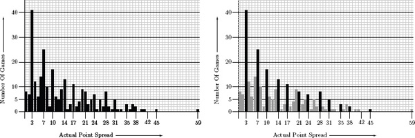
Figure 9.1 NFL 2009–2010 point-spread distribution

The graph on the right-hand side of Figure 9.1 clearly shows that the spreads in the NFL predominately spike at the 3, 7, 10, 14, 17, 21, · · · positions. This is not surprising in light of the way that points are scored in football. However, these spikes in the distribution make it difficult to accurately translate rating differences into predicted scoring differences. The best that you could reasonably hope for is to have differences in your rating system somehow pick out the most probable spike—i.e., pretend that spreads other than 3, 7, 10, 14, 17, 21, · · · are not possible and try to fit the distribution of the black bars on the right-hand side of Figure 9.1. But even if you are successful at this, you can still accumulate a large error over the course of an entire season.

Using Spreads to Build Ratings (to Predict Spreads?)

To further illustrate the issues involved in building a rating and ranking system that will reflect point spreads, let’s pretend that we have a crystal ball that allows us to look into the future so that we already know all of the spreads for all of the games in an upcoming season. Similar to Massey’s approach described on page 9, the goal is to use this information to build an optimal rating system {r₁, r₂, . . . , r_n} in which the differences r_i − r_j come as close as possible to reflecting the point spread when team i plays team j.

To do this, first suppose that in some absolutely perfect universe there is a perfect rating vector

such that each rating difference r_i − r_j is equal to each scoring difference S_i − S_j, where S_i and S_j are the respective numbers of points scored by teams i and j when they meet. If the scoring differences and rating differences are respectively placed in matrices

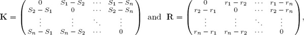
then

K = R = re^T − er^T, in which e is a column of ones.

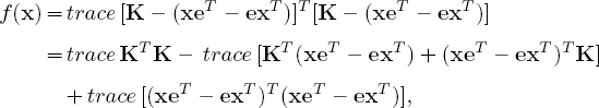
This means that in the ideal case the score-differential matrix K is a rank-two skew symmetric matrix—it is skew symmetric because k_ij = −k_ji implies that K^T = −K, and the rank is two because rank(re^T − er^T) = 2 provided that r is not a multiple of e (i.e., provided R ≠ 0). But we don’t live in a perfect universe, so, as suggested in [33], the best that we can do is to construct a ratings vector r that minimizes the distance between the score-differential matrix K and the rating-differential matrix R = re^T − er^T. This is equivalent to finding a vector x such that

is minimal for some matrix norm. The choice of the norm is somewhat arbitrary, so let’s use the simplest (and most standard) one—namely the Frobenius norm, which is

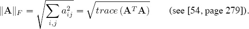
Minimizing the function f(x) in 9.1 is accomplished by using elementary calculus—i.e., look for critical points by setting ∂f/∂x_i = 0 for each i and solving the resulting system of equations for x₁, x₂, . . . , x_n. The trace function has the following properties.

trace (αA + B) = α trace (A) + trace (B),

and

trace (AB) = trace (BA) (see [54, page 90]).

Using these properties yields

so the skew symmetry of K implies that

f(x) = trace (K^TK) − 4x^TKe + 2n(x^Tx) − 2(e^Tx)².

Since ∂x/∂x_i = e_i, differentiating f with respect to x_i produces

and setting ∂f/∂x_i = 0 gives us

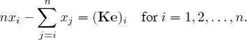
This is simply a system of linear equations that can be written as the matrix equation

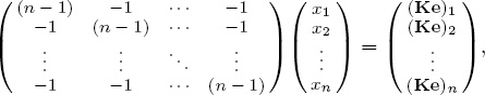
or equivalently,

Because e^TKe is a scalar and K^T = −K, it follows that

e^T Ke = (e^TKe)^T = e^TK^Te = −e^TKe e^TKe = 0,

so the vector x = Ke/n is one solution for the system in (9.2). Moreover, it can be shown that

so all solutions of the system (9.2) are of the form

By imposing some reasonable constraint, such as forcing the ratings to sum to zero, the scalar α can be evaluated, and thus a unique solution is determined. Indeed, if we require that 0 = ∑x_i = e^Tx, then

and thus

(which is the centroid (or mean) of the columns in K)

is the only critical point for f(x) that satisfies the constraint e^Tx = 0. Recall that being a critical point is only a necessary condition for being a point at which a relative minimum or maximum is attained, so we still have to check to see if r = Ke/n is indeed a minimizer. A sufficient condition for a critical point to provide a local minimum is for the Hessian [54, page 570] to be positive definite at the point, but, unfortunately, the Hessian for the case at hand is only positive semidefinite, so some additional work is required. To verify that

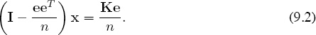
is attained at r = Ke/n, consider points in a neighborhood of r that satisfy the constraint. That is, consider r + ε, where ε ≠ 0 but e^Tε = 0, and write

The Cauchy–Schwarz (or CBS) inequality [54, page 287] says that e^Tε ≤ ||e||₂ ||ε||₂ with equality holding if and only if ε = αe for some α. Equality cannot hold for our problem because e^Tε = 0 and ε ≠ 0, so applying CBS to (9.3) leads to the conclusion that

f(r + ε) − f(r) > 0.

Therefore, the “best” ratings vector determined by point spreads is r = (Ke)/n. Below is a summary of these observations.

NFL 2009–2010 Spread Ratings

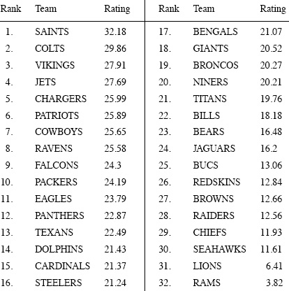
To illustrate the use of the spread ratings in (9.4), let’s use the actual score differences that occurred in the 267 games in the 2009–2010 NFL season. If teams i and j met more than once, then matrix K is constructed by letting S_i and S_j be the respective average number of points that the teams score. The resulting spread ratings are shown below.

NFL 2009–2010 spread ratings

These spread ratings correctly pick the winners in 191 out of the 267 NFL games in the 2009–2010 season for a hindsight prediction percentage of 71.54%. This is pretty good for such a simple technique—all that is required is just averaging the score differences (i.e., computing the row sums of K and dividing by 32).

Just how well do these spread ratings do in estimating the actual point spreads? The discussion on page 116 has already explained why we shouldn’t have high expectations, but let’s nevertheless have a look. The spread ratings do not take home field advantage into account, so, to be fair, we should allow home-field advantage factors to be included. Use linear regression to let the ratings determine the optimal “home-field advantage” parameters, α, β, and γ by using the linear model

where r_h and r_a are the respective ratings for the home and away teams. The parameters, α, β, and γ are determined by computing the least squares solution to the system of equations

α + βr_hi − γr_ai = S_hi − S_ai, i = 1, 2, . . . , 267

where r_hi and r_ai are the respective ratings for the home and away teams in game i, and S_hi and S_ai are the respective scores made by the home and away teams in game i. In terms of matrices this boils down to computing the least squares solution for the linear system Ax = b, or, equivalently, the solution of the 3 × 3 system of normal equations A_TAx = A^Tb, where

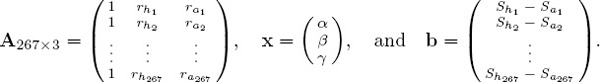
Our computer says that α = 2.3671, β = 2.4229, and γ = 2.2523, (rounded to five significant places), so estimating the point spread for each game is accomplished by setting

Estimated [(home score) − (away score) for game i] = 2.3671 + 2.4229r_hi − 2.2523r_ai.

The total absolute-spread error is the absolute deviation between the estimated score differences and the actual score differences for the entire season, and it is calculated to be

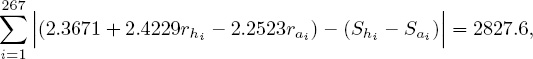
which turns out to be 10.59 points per game. To get a sense of how good or bad this is, some comparisons with other respected systems along with the actual Vegas lines might be considered.

Some Shootouts

Perhaps two of the best known and most widely respected raters are Jeff Sagarin who has been providing sports ratings for USA Today since 1985 and Ken Massey (Chapter 2) who is a contributor to the BCS college football rating system. Their respective final 2009–2010 NFL ratings that are shown below were taken from the following sites that were active at the time of this writing.

     www.usatoday.com/sports/sagarin/nfl09.htm
     www.masseyratings.com

NFL 2009–2010 Sagarin ratings

NFL 2009–2010 Massey ratings

Sagarin and Massey are short on details (most raters don’t want you to know all of the secret ingredients in their magic potions), but Sagarin states that his ratings represent a “synthesis” of two systems—an Elo system as described in Chapter 5 on page 53 that takes only winning and losing into account and some other unspecified system that considers scoring margins. Massey says that his ratings are computed as maximum likelihood estimates and are somehow tempered by a Bayesian correction—his description is too vague to implement. However, the reason that Sagarin and Massey have been singled out for comparison is because of their visibility and the fact that they have established a good record over the course of many seasons.

The results of the 2009–2010 NFL season are used below in (9.6) to compare hindsight win accuracy (percentage) and spread errors (average points per game) for six rating systems—the spread or centroid ratings on page 120; Sagarin ratings on page 122; Elo ratings on page 58; Keener ratings on page 44; Massey ratings on page 122; and, for the sake of curiosity, we also included the results derived from the Vegas betting lines that were published daily in the Raleigh, NC News and Observer. To make hindsight predictions from Sagarin’s ratings, we added 2.96 for the home team (his suggestion). Hindsight predictions for the other systems were obtained from the linear model described in (9.5) on page 121, (although Massey suggests something more complicated for his system).

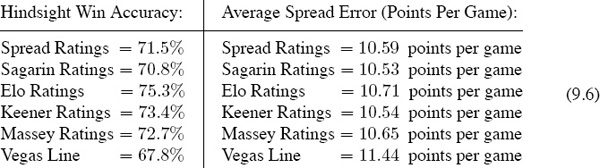
Comparisons of six rating systems using the 2009–2010 NFL season

As (9.6) shows, the hindsight accuracy for both wins and spreads of the five rating systems are all in the same ball park while the Vegas line lags slightly behind. A point being made here is that the spread (or centroid) ratings are competitive with the others for reflecting relative overall strength, but when we take into account that spread (or centroid) ratings are trivial to compute (you could do it on the back of an envelope), it makes them particularly attractive, and this is what sets the centroid method apart from other rating systems.

The performance of the Vegas line as reflected at the bottom of table (9.6) may look odd to you, but it’s not when you consider it in the proper perspective. As explained on page 113, spreads published by bookmakers are not intended to reflect or predict actual spreads or winners. Nor do bookmakers care about making a statement about the overall relative strength of each team at the end of a season, which is contrary to other rating and ranking systems that may be involved in making final BCS rankings or seeding NCAA basketball tournaments. In other words, all bookmakers care about is looking ahead to the next game of the season, so hindsight accuracy is not a goal. The foresight accuracy of the Vegas lines are typically better than their hindsight accuracy, which is not surprising because betting lines tend to reflect the combined wisdom of a large and diverse pool of people who are focused on a single upcoming game. For example, while the hindsight win accuracy for the Elo system in (9.6) is significantly better than that of the Vegas lines, the Vegas lines beat Elo in foresight accuracy. Recall from page 62 that for the 2009–2010 NFL season the foresight win accuracy for the Vegas lines was 67.8%, whereas the foresight accuracy of the Elo system was slightly smaller at 65.9%.

There is no shortage of NFL ratings (or any other kind of ratings) available on the World Wide Web, and a Google search will reveal more than what most people will care to digest. The trouble with sports ratings that are available on the Web is that they generally do not provide enough technical details to be helpful in learning how they were created or in helping you design your own system. The information in the many articles cited in the Epilogue on page 225 also hints at the vast amount of effort that has been devoted to sports ratings, but these articles are more specific for those who crave more details. If you are interested in comparisons of rating systems other than those that we have highlighted, then look at Todd Beck’s prediction tracker site

     www.thepredictiontracker.com/nflresults.php

(which was active at the time of this writing). This site shows that there is remarkable little difference in the performance of the better NFL rating systems—i.e., it is hard to stand out.

Other Pair-wise Comparisons

If you understood the derivation that produced the spread (or centroid) ratings (9.4), then it may have occurred to you that the “spreads” k_ij in the matrix K on page 118 can be interpreted more broadly than simply as scoring differences. For example, setting

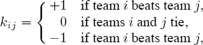
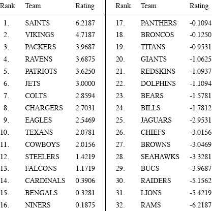
is a more basic pair-wise comparison of teams i and j than that provided by scoring differences, but K nevertheless remains skew symmetric, and exactly the same analysis holds to provide “spread ratings” r = Ke/n in a more general sense. This interpretation produces the following “win-loss” spread ratings for the 2009–2010 NFL season.

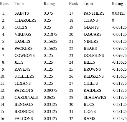
NFL 2009–2010 win-loss spread ratings

Naturally, these win-loss spread ratings are a more coarse assessment than those provided by score differences, but they nevertheless afford some information. For example, measured by the ability to win games, these ratings indicate that the CHARGERS and COLTS were on par with each other. Similarly, the EAGLES and PACKERS were indistinguishable, as were the COWBOYS, JETS, RAVENS, STEELERS, and TEXANS. And there are clearly other teams that group together in winning ability.

Depending on what you are rating or ranking, there are countless other ways to make pair-wise comparisons. For example, some situations might be better analyzed by setting k_ij = S_i/S_j, or even k_ij = log(S_i) − log(S_j). You are only limited by your imagination.

Conclusion

The next time you see a point spread published in a betting line, remember that the person, casino, or whoever is taking the bet doesn’t necessarily believe the favored team is that many points better than the underdog, but rather that they are betting on the expectation that their “predicted” point spread will generate an equal amount of money wagered on each team in the contest.

Perhaps the larger lesson is to not put an undue amount of faith in anyone’s rating system for the purpose of predicting point spreads (or even picking winners)—you would be expecting too much from a single list of numbers. If after noting this you still want to make ball-park spread predictions, then simply averaging past scoring differences as described in (9.4) on page 120 will probably give you an estimate that is competitive with more complicated techniques.

 

 

 

 

 

¹This is a Yiddish slang term derived from the Russian word “vyigrysh” for winnings or profit.

²Charles K. McNeil (1903–1981) studied mathematics at the University of Chicago where he earned a master’s degree. He went on to have at least three different careers—he taught mathematics at the Riverdale Country School, a toney prep school in New York City where John F. Kennedy was one of his students, he was a securities analyst in Chicago, and he operated his own bookmaking operation in the 1940s. His concept a of betting against a published spread changed sports wagering forever.