
Chapter Fifteen
Rank Aggregation–Part 2
The rank-aggregation methods of the previous chapter are heuristic methods, meaning that they come with no guarantees that the aggregated ranking is optimal. On the other hand, the great advantage of these heuristic methods is that they are fast, very fast compared to the optimization method of rank aggregation described in this chapter. Of course, the extra time required by this optimization method is often justified when accuracy is essential.
We now describe one optimal rank-aggregation method, which was created by Dr. Yoshitsugu Yamamoto of the University of Tsukuba in Japan [50]. This method produces an aggregated ranking that optimizes the agreement or conformity among the input rankings. There are several ways to define the agreement between the lists but one possibility creates the constants
![]()
If there are n items in total among the k input lists, then C is an n × n skew-symmetric matrix of these constants. C matrix can be formed to handle input lists that contain ties in their rankings. In addition, C can be formed for input lists that are either full or partial.
Armed with a matrix C of constants that measures conformity, our goal is to create a ranking of the n items that maximizes this. In order to accomplish this goal, we define decision variables xij that determine if item i should be ranked above item j. In particular,
![]()
To understand the use of the matrix X, consider a small example with n = 4 items labeled 1 through 4 and ranked in that order. Then the matrix X associated with this ranking is
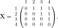
which indicates that item 1 is ranked above items 2, 3, and 4, while item 2 is ranked above items 3 and 4, and finally, item 3 is ranked above only item 4. In this example, the nice stair-step structure of X clearly reveals the ranking. At first glance, for other examples, it may not be as clear. Consider the ranking of items from first place to last place given by [4, 2, 1, 3] with the corresponding matrix
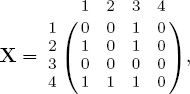
which is simply a reordering of the nice stair-step form. That is, reordering X according to the rank ordering of [4, 2, 1, 3] produces
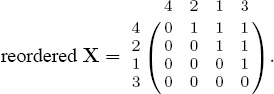
Fortunately, there is no need to actually reorder the matrix X resulting from the optimization because it is very easy to identify the ranking from the unordered X. Simply take the column sums of X and sort them in ascending order to obtain the ranking.1
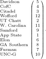
With X well understood, we now return to the optimization problem. We want to maximize conformity among the input lists, which, in terms of our constants cij and variables xij becomes
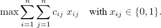
However, we must add some constraints that force the matrix X to have the properties that we observed and exploited in the small 4 × 4 example above. This can be accomplished by adding constraints of two types:
![]()
The first constraint is an anti-symmetry constraint, which says that exactly one of xij and xji can be turned “on” (i.e., set equal to 1). This captures the fact that there are only two choices describing the relationship of i and j: either i is ranked above j or j is ranked above i. The second constraint is a very clever and compact way to enforce transitivity. That is, if xij = 1 (i is ranked above j) and xjk = 1 (j is ranked above k), then xik = 1 (i is ranked above k). Transitivity is enforced by the combination of the Type 1 and Type 2 constraints. Because the decision variables are binary, the Type 2 constraint forbids cycles of length 3 from item i back to item i. The Type 1 constraint forbids cycles of length 2. In fact, these two constraints combine to forbid cycles of any length. A dominance graph helps explain this.
The matrix X from our 4 × 4 example,

can be alternatively described with the dominance graph of Figure 15.1. Every ranking
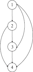
Figure 15.1 Dominance graph
vector produces a graph of this sort, which shows the dominance of an item over all items below it. The dominance graph for every ranking vector will contain no upward arcs as an upward arc corresponds to a cycle, i.e., a violation of Type 2 transitivity constraints. To see how the Type 1 and 2 constraints combine to forbid any cycles, consider the cycle from 1 → 3 → 4 → 1, which corresponds to the Type 2 constraint x13 + x34 + x41 ≤ 2. Because item 1 is ranked above item 3, x13 is turned on (i.e., x13 = 1). Similarly, x34 = 1. Then according to the Type 2 constraint, x41 must equal 0. Combining this with the Type 1 constraint, then x14 must equal 1, and thus, transitivity is enforced. In summary, all three types of constraints (Type 1 and Type 2 plus the binary constraint on xij) combine to produce an X matrix solution that is a simple reordering away from the stair-step form. Finally, because X is always a reordering of the stair-step matrix, it has unique row and column sums, and thus, produces a unique ranking of the n items. The complete binary integer linear program (BILP) is
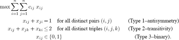
Our BILP contains n(n − 1) binary decision variables, n(n − 1) Type 1 equality constraints, and n(n − 1)(n − 2) Type 2 inequality constraints. The O(n3) Type 2 constraints dramatically limit the size of ranking problems that can be solved with this optimal rank-aggregation method. Fortunately, there are some strategies for sidestepping this issue of scale—see the respective sections on constraint relaxation and bounding on pages 190 and 191.
The Running Example
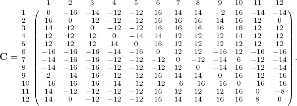
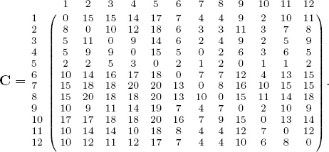
In this chapter we deviate from our usual 5 × 5 running example and introduce another slightly bigger 12 × 12 example. This example, which comes from the 2008–2009 Southern Conference (SoCon) basketball season, contains some interesting properties that the 5 × 5 example does not. In particular the SoCon example is more appropriate because it contains ties, which is the subject of the section on multiple optimal solutions on page 187.
In this section, we aggregate the rankings created by 16 different methods. For the input methods, we used the Colley, Massey, Markov, and OD methods, each with various weightings. Using the definition for conformity from Equation (15.1), the C matrix is
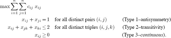
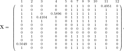
Solving the BILP produces an optimal objective value of 870 with the solution matrix X below.
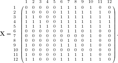
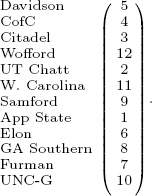
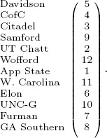
Sorting the column sums of X in ascending order ranks the twelve SoCon teams as
Solving the BILP
BILPs are typically solved with a technique called branch and bound, which uses a series of linear programming (LP) relaxations of the problem to form a tree to narrow down the process of stepping through the discrete solution space. Because discrete optimization is much harder than continuous optimization, the size of the problem, becomes an issue. Remember the size of the problem is governed by n, the number of items being ranked. Our rank-aggregation BILP contains n(n − 1) binary decision variables as well as n(n − 1) Type 1 constraints and n(n − 1)(n − 2) Type 2 constraints. The O(n3) number of constraints dramatically limits the size of the ranking problem that can be handled by this optimal conformity method. In contrast, the heuristic method of the previous chapter had no such scalability issues. Fortunately, there are some very clever strategies for sidestepping this scale issue, as the discussion in the sections on pages 190 and 191 show.
Multiple Optimal Solutions for the BILP
The branch and bound procedure terminates with an optimal solution X. As we saw with our small examples, finding and sorting the column sums in ascending order gives the optimal ranking of the items. Problem solved—we can pack up and go home. Not if you are a mathematician. Mathematicians like to ask deeper questions, such as: is the optimal solution unique? If not, can we find alternate optimal solutions?
It turns out that these questions have answers that reveal hints for circumventing the scalability issues mentioned above. There is a simple test to determine if the optimal solution to the BILP is unique. Consider each successive pair of items in the optimal ranked list and ask if the two items i and j can be swapped without changing the objective value. Only swaps of rank neighboring items need be considered as these are the only swaps that do not violate the constraints. The objective value will not change if cij = cji. If this is so, then an alternate optimal solution is one that has these two items swapped. There may indeed be more than a two-way tie at this rank position. For instance, a three-way tie occurs if cij = cji = cik = cki = cjk = ckj for rank neighboring items i, j, and k. Continue down the optimal ranked list in this fashion detecting any two-way or higher ties at each position. We apply this Tie Detection algorithm to the SoCon example. From the running example on page 185, the BILP produced the optimal ranking of
We begin the Tie Detection algorithm by comparing the two teams at the top of the list. Because C(5, 4) ≠ C(4, 5), these two cannot be swapped. Thus, we move onto the next pair of teams in the ranked list, teams 4 and 3. Because C(4, 3) ≠ C(3, 4), these two cannot be swapped either. We move down the list to teams 3 and 12, which again cannot be swapped. Finally, we reach a pair that can be swapped, the pair of 12 and 2. This means that teams 12 and 2 can appear in either order in the optimal ranked list, with 12 above 2 as the BILP algorithm found or with 2 above 12, which is an alternate optimal solution since the objective function is unchanged yet feasibility is still maintained. At this point, we have discovered a two-way tie between teams 12 and 2, but a three-way or higher tie may exist. So we check to see if the next team in the list, team 11, satisfies C(12, 2) = C(2, 12) = C(2, 11) = C(11, 2) = C(12, 11) = C(11, 12), which it does not. Thus, the tie at the fourth rank position is indeed only a two-way tie between teams 12 and 2. We continue down the list, considering 11 and 9, then 9 and 1, and so on, and we find no more ties. As a result, this SoCon example has two integer optimal solutions and infinitely many fractional optional solutions on the boundary between these two.
In summary, we know that we can (1) apply a branch and bound procedure to find an optimal solution to the rank-aggregation BILP, (2) check the uniqueness of the obtained optimal solution, and (3) if applicable, find several alternate optimal solutions with the simple O(n) test described above. As a result, this optimization technique produces an output ranking that may actually contain ties and is a very mathematically appealing and provably optimal ranking method. However, the BILP is much slower than many existing rating and ranking methods. In fact, because of the O(n3) constraints, in practice, a commercial BILP solver such as the DASH Optimization software or the NEOS server is limited to a problem with about a thousand items. Thus, ranking all NCAA Division 1 football or basketball teams is certainly within reach while ranking billions of webpages in cyberspace is not. Yet ranking the top 50 results produced by several popular search engines is not only possible, but fast—as it can be done in real-time. Fortunately, the next section explains how we can further increase the practical limit on n, making the aggregated ranking of several thousand items possible.
The LP Relaxation of the BILP
The first step to solving a big nasty BILP is to solve a related problem, the relaxed LP. For us, this means relaxing the Type 3 constraints that force the variables xij to be discrete, specifically, binary since xij ![]() {0, 1}, and allow them to be continuous so that 0 ≤ xij ≤ 1. Actually, the upper bound of the bound constraint 0 ≤ xij ≤ 1 is redundant as this restriction is covered by the Type 1 constraint xij + xji = 1. Thus, the simplified relaxed LP for the rank-aggregation problem is
{0, 1}, and allow them to be continuous so that 0 ≤ xij ≤ 1. Actually, the upper bound of the bound constraint 0 ≤ xij ≤ 1 is redundant as this restriction is covered by the Type 1 constraint xij + xji = 1. Thus, the simplified relaxed LP for the rank-aggregation problem is
When some BILPs are solved as LPs the optimal solution to the relaxed problem, the LP, gives a solution with binary values, which is clearly also optimal for the BILP. This is the best-case scenario. The next best scenario is when the optimal solution for the LP contains just a small proportion of fractional values. Often, in this case, these few fractional values can be rounded to the nearest integer giving a slightly suboptimal solution that, if feasible, may adequately approximate the exact optimal integer solution. In this section, we show that the LP gives very interesting results. Many times the LP solution is optimal and, in fact, readily tells us all alternate optimal solutions as well.
Our 12-team SoCon example makes this point well. We discovered in the section on multiple optimal solutions on 187 that this example has two integer optimal solutions. One with the teams in the rank order given by (5 4 3 12 2 11 9 1 6 8 7 10) and the other with teams 12 and 2 switched. Notice how this tie is manifested in the LP solution matrix X below.
The LP solution contains fractional values in locations X(12, 2) and X(2, 12), precisely the locations in C that indicated a tie between teams 12 and 2. The LP solver has terminated with a fractional optimal solution and this solution lies on the boundary between the two integer optimal solutions of the BILP. Because the LP terminated with the identical optimal objective value, 870, that the BILP has, we know the LP solution is optimal for the original BILP.
Though the above SoCon example ends in a fractional solution from which optimal binary solutions can be constructed, this is not guaranteed. In fact, we constructed a 9-item example with a unique fractional optimal solution. Thus, when binary solutions are constructed, the objective value is not as good as that produced by the unique fractional solution. However, this example with a unique fractional solution was hard to construct. In fact, to locate such an instance, we randomly generated thousands of C matrices with entries uniformly distributed between −1 and 1 before we encountered the unique fractional 9-item example. Thus, though unique fractional solutions are possible, it is more likely in practice that the relaxed LP formulation of our ranking problem will result in non-unique fractional solutions from which multiple optimal binary solutions can be constructed. Empirical studies by Reinelt et al. [62, 65, 64, 63] add further evidence that the LP results for ranking problems are exceptionally good and often optimal and binary in practice.
In which cases can we be certain that the optimal LP solution is also optimal for the BILP? Remember, after all, that the BILP is truly the problem of interest for us. Of course, if the LP solution is binary, then that solution is optimal for the BILP. But even when the LP solution is fractional, there are instances in which it is optimal for the BILP as the SoCon example showed. In [50], Langville, Pedings, and Yamamoto proved conditions that identify when an LP solution is optimal for the BILP. Their theorem also connects the presence of multiple optimal solutions for the BILP, which indicate the presence of ties in the ranking, to fractional values in the LP solution.
Their theorem carries computational consequences as well. The original LP solver, the famous simplex method, is not the method of choice for solving our MVR problem. The simplex method is an extreme point method, meaning that it moves from one extreme point to the next, in an ever-improving direction until it reaches an optimal solution, which will, of course, also be an extreme point. In contrast, interior point LP solvers move through the interior of the feasible region until they converge on an optimal solution that may be an extreme point or a boundary point depending on the path taken through the interior of the feasible region. For us, it is the boundary optimal points (which contain fractional values) that give us so much more information than extreme optimal points (which are the integer-only solutions). Thus, we always choose a non-extreme point, non-simplex LP solver when solving the relaxed LP associated with the ranking problem.
Constraint Relaxation
Even with the LP relaxation, the O(n3) Type 2 constraints drastically limit the size of the ranking problems that we can handle. So we must resort to another relaxation technique, constraint relaxation, to increase the size of tractable problems. Of the n(n − 1)(n − 2) Type 2 constraints, xij + xjk + xki ≤ 2, only a very small proportion of these are necessary. The great majority of these will be trivially satisfied—the problem is that we don’t know which are necessary and which are unnecessary. In order to find out, we start by assuming all are unnecessary, then slowly add back in the necessary ones as they are identified. The Type 1 and relaxed continuous version of the Type 3 constraints cause no problems, so we leave these unchanged. Below are the steps involved in the constraint relaxation technique. Constraint relaxation can be applied with equal success to either the BILP or the LP. We have chosen to describe it for the BILP only.
CONSTRAINT RELAXATION ALGORITHM FOR LARGE RANKING BILPS
1. Relax all Type 2 constraints so that the initial set of necessary Type 2 constraints is empty.
2. Solve the BILP with the current set of necessary Type 2 constraints. Form the optimal ranking associated with this solution. This ranking is actually an approximation to the true ranking we desire for the original problem with the full Type 2 constraint set.
3. Determine which Type 2 constraints are violated by the solution from Step 2—these are necessary Type 2 constraints. Add these Type 2 constraints to the set of necessary Type 2 constraints and go to Step 2. Repeat until no Type 2 constraints are violated. The BILP solution at this point is an optimal ranking for the original problem with the full constraint set.
In Step 3, the determination of which Type 2 constraints are violated by the current BILP solution is easy and does not require that each constraint be checked one by one. Recall from Figure 15.1 that violations to the Type 2 transitivity constraints are upward arcs in the dominance graph. In yet another view, these violations manifest as ones on the lower triangular part of the rank reordered matrix X. For each identified upward arc (j, i), next find all k such that xik = xkj = 1 and generate the corresponding Type 2 constraint xji + xik + xkj ≤ 2. The matrix X can be used to quickly find these elements k: form the Hadamard (element-wise) product of the ith row and jth column of X. All nonzero elements in this product satisfy xik = xkj = 1. Because of the upper triangular structure of the reordered matrix X, it takes much less than O(n) work to compute the Hadamard product and form the transitivity constraints associated with each upward arc.
In addition, we can take advantage of any approximate rankings that may exist. For example, suppose a fast heuristic method is run and a ranking produced. This ranking has a one-to-one correspondence to a matrix, let’s call it ![]() , in upper triangular form. Computing the objective value f(
, in upper triangular form. Computing the objective value f(![]() ) = C.
) = C. ![]() for this approximate solution matrix
for this approximate solution matrix ![]() gives a useful lower bound on the objective. As the branch and bound BILP procedure explores solutions and encounters a branch with nodes having value below f(
gives a useful lower bound on the objective. As the branch and bound BILP procedure explores solutions and encounters a branch with nodes having value below f(![]() ), nodes in that branch no longer need to be explored.
), nodes in that branch no longer need to be explored.
In summary, the constraint relaxation technique is an iterative procedure that solves a series of BILPs whose constraint set gradually grows until all the necessary transitivity constraints are identified. At each iteration the optimal BILP solution is an approximation to the true optimal ranking of the original problem with the full constraint set. The approximations improve until the optimal ranking is reached.
Sensitivity Analysis
Another advantage of the LP over the BILP relates to the natural sensitivity measures produced when solving a linear program. In this case, we are interested in changes in the objective coefficients cij. Slight changes in the input data (specifically the differential matrix D that creates the objective coefficient matrix C) could change the optimal solution, and hence, optimal ranking of the teams. Industrial optimization software, such as Xpress-MP, computes the following ranges given in Figure 15.2 on the objective coefficients for the 12-team SoCon example.
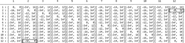
Figure 15.2 Sensitivity ranges on the objective coefficients cij
Most cij coefficients have very loose bounds. In fact, the only entries with finite ranges are the pair of 2 and 12. For this dataset, these ranges warn us that we are less certain of the rank ordering of these two teams in the middle of the pack, which are the same two teams that, in the section on multiple optimal solutions on 187, we found are tied in the ranking. Changes of the objective coefficients outside of the given ranges, can change the ranking.
Bounding
Bounding techniques are extremely useful in optimization. In particular, solution techniques for integer programs rely heavily on bounding. In this section, we apply such bounding to the Iterative LP method to accelerate convergence and produce optimality guarantees. Recall that the Iterative LP method relaxes the transitivity constraint set. In fact, at the first iteration, the LP is solved with no transitivity constraints. The optimal solution matrix X at this iteration creates an objective function value that we denote ![]() since it is an upper bound of the optimal objective value f*. The solution at this iteration almost always violates some transitivity constraints and thus is not a feasible solution for the original LP. However, it can be used to form a very useful approximate solution. This is done by computing the row sums of X. The ith row sum is a good indicator of how many opponents the ith team will beat. As the iterative LP method proceeds, we use the row sums of each iteration’s solution matrix X to compute an approximate ranking. This approximation gets closer to the optimal ranking as the iterations proceed. Because every ranking, including these approximate ones, has a one-to-one correspondence with an X matrix, we can compute the objective function value for each approximate ranking, which we denote f since it is a lower bound of f*. Thus, we know that
since it is an upper bound of the optimal objective value f*. The solution at this iteration almost always violates some transitivity constraints and thus is not a feasible solution for the original LP. However, it can be used to form a very useful approximate solution. This is done by computing the row sums of X. The ith row sum is a good indicator of how many opponents the ith team will beat. As the iterative LP method proceeds, we use the row sums of each iteration’s solution matrix X to compute an approximate ranking. This approximation gets closer to the optimal ranking as the iterations proceed. Because every ranking, including these approximate ones, has a one-to-one correspondence with an X matrix, we can compute the objective function value for each approximate ranking, which we denote f since it is a lower bound of f*. Thus, we know that
![]()
Next we bound the relative error ![]() associated with the approximate ranking. Because f, f*, and
associated with the approximate ranking. Because f, f*, and ![]() all have the same sign, we can bound the relative error, which involves the unknown f* with the known quantities f and
all have the same sign, we can bound the relative error, which involves the unknown f* with the known quantities f and ![]() .
.
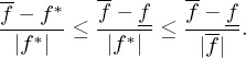
Further, when all elements of the objective coefficient matrix C are integral and ![]() − f ≤ 1, the approximate ranking is the optimal solution of the original ranking problem. Even when we are not so lucky as to be able to guarantee optimality, we can give a guarantee on the error associated with the near-optimal solution. We can guarantee that the optimal objective value is between f and
− f ≤ 1, the approximate ranking is the optimal solution of the original ranking problem. Even when we are not so lucky as to be able to guarantee optimality, we can give a guarantee on the error associated with the near-optimal solution. We can guarantee that the optimal objective value is between f and ![]() and the relative error is not greater than
and the relative error is not greater than ![]() . This is another great advantage of the bounding version of our Iterative LP method. Not only does it require fewer iterations but it also allows the user to stop the iterative procedure as soon as an acceptable relative error is reached.
. This is another great advantage of the bounding version of our Iterative LP method. Not only does it require fewer iterations but it also allows the user to stop the iterative procedure as soon as an acceptable relative error is reached.
ASIDE: Ranking in Rome
Throughout this book we have emphasized the many and varied uses of the ranking methods described. Perhaps one of the most unlikely and little known uses is archaeology. Picture the large excavation sites of Pompeii or Rome, Italy. The phrase “when in Rome, rank” is good advice for an archaeologist hoping to correctly date items from a dig. A typical dig is divided into several sites at which excavation is done. At each site, recovered items are carefully tagged according to the depth from which they were unearthed. Multiple styles of pottery or classes of artifacts are discovered at multiple sites at multiple dig depths. The archaeologist’s goal is to determine the relative age of a class of artifact. For instance, for transporting water, did the Romans first use painted clay vases or mosaic mud jugs? At one dig site the vase may have appeared at a lower dig depth than the jug, suggesting the vase came first. The order may be reversed at another site. In effect, each site creates a ranking of the items according to their dig depth. The goal is to determine the overall ranking of the artifacts that is most consistent with all sites. Mathematically, we want to aggregate the rankings from each site into an optimal ranking that maximizes agreement among the many sites.
Summary of the Rank-Aggregation (by Optimization) Method
The shaded box below assembles the labeling conventions we have adopted to describe our optimal rank-aggregation method.
Notation for the Rank-Aggregation (by Optimization) Method
n number of items to be ranked
C conformity matrix with coefficients of objective function
The list below summarizes the steps of the rank-aggregation method.
RANK-AGGREGATION (BY OPTIMIZATION) METHOD
1. Form the matrix C according to some conformity definition. For example,
cij = (# of lists with i above j) − (# of lists with i below j).
2. Solve the LP optimization problem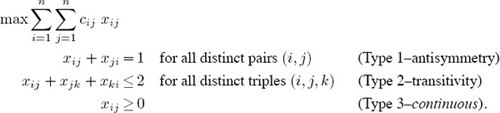
For problems with large n, use the constraint relaxation and bounding techniques discussed in the sections on pages 190 and 191.
3. The optimal ranking is produced by sorting the columns of the optimal solution matrix X in ascending order. Ties in the ranking are identified by the location of fractional values in X.
We close this section with a list of properties of this rank-aggregation method.
• Our experiments show that when the lists to be aggregated are largely in agreement from the start, then only a handful of iterations are required. This is very good news if you are in the business of building a meta-search engine that aggregates the top-100 results from five popular search engines. Our rank-aggregation methods can be executed in just a few seconds on the latest laptop machine.
• The constraints of the simplified relaxed LP create a polytope that has been well-studied and is often referred to as the linear ordering polytope [65]. It is helpful to study the relationship of the LP’s polytope to the feasible region of the original BILP. Of course, the feasible region of the BILP is contained within the feasible region of the LP. The best scenario is when the LP’s feasible region is as tight as possible to the BILP’s feasible region. In other words, the LP’s feasible region is the convex hull of the points in the BILP’s feasible region. For our ranking problem, the good news is that all of the inequality constraints (Type 2 transitivity and Type 3 nonnegativity) are facet-defining inequalities for the linear ordering polytope. This means that these inequalities are as tight as possible. However, the set of constraints for the LP does not cover all facet-defining inequalities for the linear ordering polytope. Sophisticated valid inequalities such as the so-called fence and Mobius ladder inequalities create stronger LP relaxations, but unfortunately they are too costly to generate [57, 62, 64].
• LPs come with the wonderful capability of sensitivity analysis. That is, LPs are amenable to “what if” scenario analysis. When certain input parameters are changed, we can determine if the optimal solution changes and by how much. Because we have shown that an LP can be used to solve the ranking problem, then there is the potential for sensitivity analysis. In this case, we can answer questions about how changes in the objective coefficients cij affect the optimal solution. Such sensitivity analysis is additional information that few, if any, other ranking methods deliver.
Revisiting the Rating-Differential Method
In Chapter 8, we described the rating-differential method for ranking items. That method aims to find a reordering of the items that when applied to the item-item matrix of differential data forms a matrix that is as close to the so-called hillside form as possible. The following figure summarizes the concept pictorially.
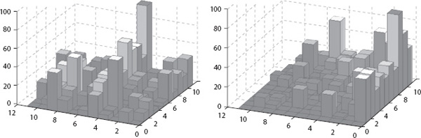
On the left is a cityplot of an 11 × 11 matrix in its original ordering of items, while the right is a cityplot of the same data displayed with the new optimal ordering. The cityplot on the right resembles a hillside as the ordering was chosen to bring the matrix as close to hillside form as possible.
Rating Differential vs. Rank Aggregation
In Chapter 8 we formulated an optimization problem whose objective was to minimize the (possibly weighted) count of the number of violations from the hillside form defined in the box on page 108. In that chapter, we described an evolutionary approach to solving this optimization problem. In this section, we show that the rating-differential optimization problem can actually be solved optimally and efficiently with the techniques of this chapter. Much of the work for this section was developed in [50], where we referred to the method as the Minimum Violation Ranking (MVR) method, since it produces a ranking that minimizes hillside violations.
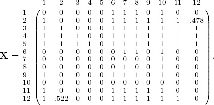
In fact, the rating-differential method fits exactly into the BILP, and thus, LP, formulation of this chapter. Let’s focus on the data matrix D of point differentials, wherein dij is the number of points winning team i beat losing team j by in their matchup, 0 otherwise. The trick is to think of each row and column of D as a team’s ranking of its opponents. For instance, for our 5-team example with
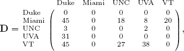
the second row of D tells us that Miami would rank its opponents’ defensive ability from strongest to weakest as UVA, UNC, VT, Duke. On the other hand, the first column of D, for example, tells us that Duke would rank its opponents’ offensive ability as Miami/VT, UVA, UNC. Consequently, these rankings, both offensive and defensive for the n teams can be aggregated to create an overall ranking for the season. The only modification to the rank-aggregation method of this chapter is in the definition of the conformity matrix C. Rather than the definition of Equation (15.1), the conformity matrix for the rating-differential method is
Definition of the C Matrix
Let C = [cij] ∀ i, j = 1, 2, . . . , n be defined as
![]()
where # denotes the cardinality of the corresponding set. Thus,
#{k | dik < djk}
is the number of teams receiving a lower point differential against team i than team j. Similarly, #{k | dki > dkj} is the number of teams receiving a greater point differential against team i than team j.
Note: The matrix C above counts hillside violations in a binary fashion, however, something more sophisticated can be done. For instance, we can consider weighted violations by summing the difference each time a hillside violation occurs. In this case, C is defined as cij := ![]() k:dik < djk (djk − dik) +
k:dik < djk (djk − dik) + ![]() k:dki > dkj (dki − dkj).
k:dki > dkj (dki − dkj).
The Running Example
This definition for C produces the following conformity matrix for the 12-team SoCon example.
Solving this example with LP formulation of this chapter produces the optimal X matrix below.
which corresponds to the ranking of teams given by
The fractional values in X indicate that there are a few ties. There is a two-way tie at the second rank position between teams 4 and 3 and another two-way tie at the sixth position between teams 11 and 1.
The box below summarizes the steps of the Minimum Violation Ranking (MVR) method.
Minimum Violation Ranking (MVR) Method
1. Form the coefficient matrix C from the differential matrix D according to the definition.2
cij := #{k | dik < djk} + #{k | dki > dkj},
2. Solve the LP optimization problem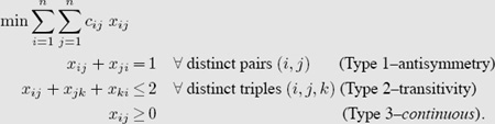
For problems with large n, use the constraint relaxation and bounding techniques discussed in the sections on 190 and 191.
3. The optimal ranking is produced by sorting the columns of the optimal solution matrix X in ascending order. Ties in the ranking are identified by the location of fractional values in X.
ASIDE: March Madness and Large LPs
In order to demonstrate the size of the LPs to which the MVR ranking techniques of this chapter can be applied, we ranked the 347 teams in NCAA college basketball for the 2008–2009 season. To solve the large MVR LP, we used the iterative constraint relaxation trick. We used the conditions of a theorem from [50] and our computational results (i.e., f(LP) = f(BILP)) to conclude that the Iterative LP method produced a non-unique fractional solution that was optimal for the original BILP.2 Just .066% of the nonzero values in the optimal LP solution are fractional. In addition, the fractional values, and hence, the ties, occurred in positions of lower rank, particularly rank positions 252 through 272.
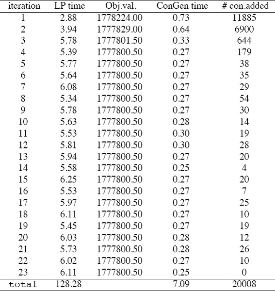
Table 15.1 shows the breakdown of how much time is spent at each iteration of the Iterative LP method for the full 347-team example. For example, at iteration 1, solving the LP required 2.88 seconds and produced an objective value of 1778224, while finding the necessary Type 2 constraints required .73 seconds and generated 11885 additional constraints to be added to the LP formulation to be solved at iteration 2. In total, executing all 23 iterations and generating all 20,008 constraints required just 135.37 seconds on a laptop machine. Another observation from Table 15.1 concerns the remarkable value of the constraint relaxation technique described on page 190. Just .048% of the total original Type 2 constraints are necessary. This is a huge savings and makes even larger ranking problems within reach. One final observation from Table 15.1 is in order. Notice that by iteration 4, the Iterative LP method has reached a solution that is on the optimal face of the feasible region, yet is infeasible. At each subsequent iteration, the solution is improved in terms of feasibility, not optimality. In other words, the solutions remain on the optimal hyperplane yet move closer to the feasible region at each iteration.
Table 15.1 Breakdown of computation for Iterative LP method on 347-team example
Next we demonstrate the improvements that are possible with the bounding version of our Iterative LP method.
Table 15.2 Computational results for Iterative LP method with bounding on 347 NCAA teams
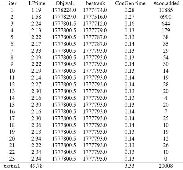
Notice that the bounding technique significantly reduced the overall run time (53.11 seconds) and terminated with a result that was not proven to be optimal, yet can be proven to be very near the optimal solution since the relative error is no greater than .000422%. We were ultimately able to conclude that this solution is indeed optimal since the Iterative BILP method returned the same objective function value as the Iterative LP method.
8th = lowest seeded team to win the NCAA basketball tournament.
— Villanova, 1985, defeated Georgetown, 66–64.
11th = lowest seeded team to to reach the Final Four.
— LSU, 1986, lost to Louisville in the semifinals.
— wiki.answers.com & tourneytravel.com
1Or the row sums sorted in descending order could be used.
2The matrix C above counts hillside violations in a binary fashion, but something more sophisticated can be done. For instance, we can consider weighted violations by summing the difference each time a hillside violation occurs, in which case, C is defined as cij := ![]() k:dik < djk (djk − dik) +
k:dik < djk (djk − dik) + ![]() k:dki > dkj (dki − dkj).
k:dki > dkj (dki − dkj).
2Using a slightly different input matrix D, a point-differential matrix based on cumulative, rather than average, point differentials produced a binary LP solution that is consequently optimal for the BILP.