
Chapter Two
Massey’s Method
The Bowl Championship Series (BCS) is a rating system for NCAA college football that was designed to determine which teams are invited to play in which bowl games. The BCS has become famous, and perhaps notorious, for the ratings it generates for each team in the NCAA. These ratings are assembled from two sources, humans and computers. Human input comes from the opinions of coaches and media. Computer input comes from six computer and mathematical models—details are given in the aside on page 17. The BCS ratings for the 2001 and 2003 seasons are known as particularly controversial among sports fans and analysts. The flaws in the BCS selection system as opposed to a tournament playoff are familiar to most, including the President of the United States—read the aside on page 19.
Initial Massey Rating Method
In 1997, Kenneth Massey, then an undergraduate at Bluefield College, created a method for ranking college football teams. He wrote about this method, which uses the mathematical theory of least squares, as his honors thesis [52]. In this book we refer to this as the Massey method, despite the fact that there are actually several other methods attributed to Ken Massey. Massey has since become a mathematics professor at Carson-Newman College and today continues to refine his sports ranking models. Professor Massey has created various rating methods, one of which is used by the Bowl Championship Series (or BCS) system to select NCAA football bowl matchups—see the aside on page 17. The Colley method, described in the next chapter, is also one of the six computer rating systems used by the BCS. Because the details of the Massey method that is used by the BCS are vague, we describe the Massey method for which we have complete details, the one from his thesis [52]. Readers curious about Massey’s newer, BCS-implemented model can peruse his sports ranking Web site (masseyratings.com) for more information.

K. Massey
Massey’s Main Idea
The fundamental philosophy of the Massey least squares method can be summarized with one idealized equation,
ri − rj = yk,
where yk is the margin of victory for game k, and ri and rj are the ratings of teams i and j, respectively. In other words, the difference in the ratings ri and rj of the two teams ideally predicts the margin of victory in a contest between these two teams.
The goal of any rating system is to associate a rating for each team in a league of n teams, where m total league games have been played thus far. Of course, we do not know the ratings ri for the teams, but we do know who played who and what the margin of victory was. Thus, there is an equation of this form for every game k, which creates a system of m linear equations and n unknowns that can be written as
Xr = y.
Each row of the coefficient matrix X is nearly all zeros with the exception of a 1 in location i and a -1 in location j, meaning that team i beat team j in that matchup. Thus, Xm×n is a very sparse matrix. The vector ym×1 is the right-hand side vector of margins of victory and rn×1 is the vector of unknown ratings. Typically, m >> n, which means the linear system is highly overdetermined and is inconsistent. All hope is not lost as a least squares solution can be obtained from the normal equations XTXr = XTy. The least squares vector, i.e., the solution to the normal equations, is the best (in terms of minimizing the variance) linear unbiased estimate for the rating vector r in the original equation Xr = y [54].
Massey discovered that due to the structure of X it is advantageous to use the coefficient matrix M = XTX of the normal equations. In fact, M need not be computed. It can simply be formed using the fact that diagonal element Mii is the total number of games played by team i and the off-diagonal element Mij, for i ≠ j, is the negation of the number of games played by team i against team j. In a similarly convenient manner, the right-hand side of the normal equations XTy can be formed by accumulating point differentials. The ith element of the right-hand side vector XTy is the sum of the point differentials from every game played by team i that season, and so we define p = XTy. Thus, the Massey least squares system becomes
Mr = p,
where Mn×n is the Massey matrix described above, rn×1 is the vector of unknown ratings, and pn×1 is the right-hand side vector of cumulative point differentials.
The Massey matrix M has a few noteworthy properties. First, M is much smaller in size than X. In fact, it is a square symmetric matrix of order n. Second, it is a diagonally dominant M-matrix. Third, its rows sum to 0. As a result, the columns of M are linearly dependent. This causes a small problem as rank(M) < n and the linear system Mr = p does not have a unique solution. Massey’s workaround solution to this problem is to replace any row in M (Massey chooses the last) with a row of all ones and the corresponding entry of p with a zero. This adds a constraint to the linear system that states that the ratings must sum to 0 and results in a coefficient matrix that is full rank. A similar trick is employed in the direct solution technique for computing the stationary vector of a Markov chain. See Chapter 3 of [75]. The new system with the row adjustment is denoted ![]() .
.
The Running Example Using the Massey Rating Method
Now create Massey ratings for the five team example on page 5. Each team played every other team exactly once, so the off-diagonal elements of M are -1 and the diagonal elements are 4. But to insure that M has full rank (and hence a unique least squares solution), use the trick suggested by Massey in [52], and replace the last row with a constraint that forces all ranks to sum to 0. Thus, the Massey least squares system ![]() is
is
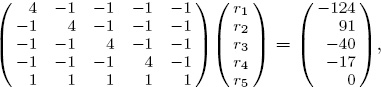
which produces the Massey rating and ranking lists given in the following table.
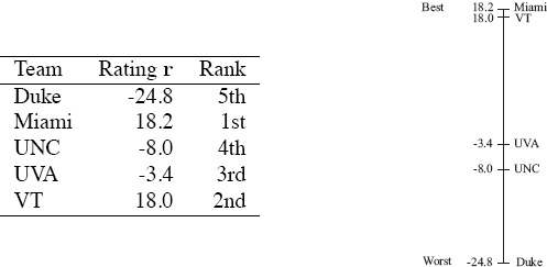
Tabular presentation of rating and ranking values is useful, but sometimes the number line representation that is shown on the right-hand side in the figure above is better. The line representation makes it easier to see the relative differences between teams, and this additional information is something we exploit in the section on rating aggregation on 176.
Advanced Features of the Massey Rating Method
These results are reasonable for this tiny dataset, yet there is more to the Massey method [52]. In fact, two vectors more. Massey creates two new vectors, an offensive rating vector o and a defensive rating vector d, from the overall rating vector r. Massey assumes that team i’s overall rating is the sum of its offensive and defensive ratings, i.e., ri = oi + di. Massey squeezes o and d from r using some clever algebra. However, in order to understand the algebra, we need some additional notation. The right-hand side vector p, whose ith element pi holds team i’s cumulative point differentials summed over all games played that season, can be decomposed into p = f − a. The vector f is the “points for” vector, which holds the total number of points scored by each team over the course of the season. The vector a is called the “points against” vector and it holds the total number of points scored against each team over the course of the season. One additional decomposition is required to understand Massey’s method for finding o and d. The Massey coefficient matrix M can be decomposed into M = T − P, where T is a diagonal matrix holding the total number of games played by each team and P is an off-diagonal matrix holding the number of pair-wise matchups between teams during the season. We begin with the original Massey least squares system Mr = p and use a string of substitutions to show how the two new rating vectors o and d are derived.
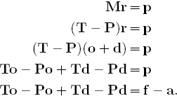
Now the final equation above can be split into two separate equations.
To − Pd = f and Po − Td = a.
The equation on the left, To − Pd = f, says that the total number of points scored by a team over the course of a season can be built by multiplying the offensive score of that team by the number of games played, then subtracting the sum of the defensive scores of its opponents. Working with the equation on the left brings us closer to solving for the two new rating vectors o and d.
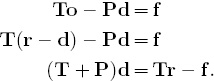
Notice that the right-hand side Tr − f from the last line above is a vector of constants as r has already been computed. Thus, the Massey linear system for finding d (given r) is
(T + P)d = Tr − f.
And finally, once both r and d are available, o can be computed using the fact that r = o + d.
The Running Example: Advanced Massey Rating Method
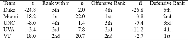
Massey’s creation and use of o and d opens an interesting avenue of research for sports ranking models. Namely, the prediction of point outcomes or at least point spreads. Thus, we apply Massey’s method to our small example. In particular, Massey uses these two new rating vectors o and d to predict point scores of future matchups. He assumes that oi gives “the number of points team i is expected to score against an average defense.” Combining this with the available defensive ratings, Massey makes point outcome predictions. In particular, if teams i and j play, then the predicted number of points team i would score against team j is given by oi − dj. Similarly, the predicted number of points team j would score against team i is given by oj − di. Table 2.1 gives all three rating vectors for the complete Massey method. Notice that the method predicts a VT vs. Duke game outcome of 20.7 − (−26.8) = 47.5 to 2.0 − (−2.7) = 4.7, or roughly 48 to 5. This is rather close to the actual game outcome from the 2005 data, as VT beat Duke 45 to 0 that year. Before getting too excited about the gambling potential of the advanced Massey model, note that not all predictions are this good. For example, the model predicts Miami to beat VT by a score of 25 to 24, which is quite far from the actual game outcome of 25 to 7 from the 2005 data. Part of the blame associated with the volatility of the predictions’ success lies with the tiny amount of data (just five teams) used. The issue of point spreads is of interest to many sports fans, particularly the betting types, so a complete discussion of point spreads and optimal “spread ratings” is presented in Chapter 9 on page 113.
Table 2.1 Complete list of Massey rating and ranking vectors
Summary of the Massey Rating Method
Shown below are the labeling conventions that have been adopted to describe the Massey method for ranking sports teams.
n number of teams in the league = order of the matrices T, P, and M
m number of games played
Xm×n game-by-team matrix;
Xki = 1, if team i won in game k, -1, if team i lost, 0, otherwise.
Tn×n diagonal matrix containing information about the total games played;
Tii = total number of games played by team i during the season
Pn×n off-diagonal matrix containing pair-wise matchup information;
Pij = number of pair-wise matchups between teams i and j
Mn×n square symmetric M-matrix called the Massey Matrix;
M = T − P
![]() n×n adjusted Massey Matrix that is created when one row of M is replaced with eT (the vector of all ones)
n×n adjusted Massey Matrix that is created when one row of M is replaced with eT (the vector of all ones)
fn×1 cumulative points for vector;
fi = total points scored by team i during the season
an×1 cumulative points against vector;
ai = total points scored against team i during the season
Pn×1 cumulative point differential vector;
pi = fi − ai; cumulative point differential of team i during the season
![]() n×1 adjusted point differential vector created when one element of p is replaced with a 0
n×1 adjusted point differential vector created when one element of p is replaced with a 0
rn×1 general rating vector produced by the Massey least squares system
on×1 offensive rating vector produced by the Massey least squares system
dn×1 defensive rating vector produced by the Massey least squares system
Massey Least Squares Algorithm
1. Solve the system ![]() to obtain the general Massey rating vector r.
to obtain the general Massey rating vector r.
2. Solve the system (T + P)d = Tr − f for the defensive rating vector d.
3. Compute the offensive rating vector o = r − d.
Listed below are some properties of the Massey method.
• The Massey method uses point score data to rate teams. However, other game statistics could be used. And in other contexts, any data on pair-wise comparisons of items could be used. For example, to rate the trading power of nations, the gross number of exports could be used. The nation with the larger number of exports (perhaps normalized by accounting for population) would win in the hypothetical matchup. In this way, the United Nations’ HDI measure of page 6 could be augmented and enhanced.
• The Massey method creates three vectors, the general rating vector r, the offensive rating vector o, and the defensive rating vector d. By cleverly combining o and d, one can estimate point spreads. (Also see Chapter 9 on page 113.)
ASIDE: The Massey Method for Ranking Webpages
In this aside we apply the Massey method to webpages to emphasize the point that this method can be used to rank any collection of items. (Actually, with just a little thought, the same is true of every method in this book.) Because webpages are presented in response to user queries based on their ranked order, webpage rankings are a fundamental part of every major search engine. For instance, Figure 2.1 shows the webpages ranked in positions 1 through 10 for a query to Google on the phrase “Massey ranking.”
The trick to applying the Massey method to the Web is to define the notion of a game or pair-wise matchup for webpages. There are numerous possibilities. For example, if statistics on webpage traffic are available with the Alexa search engine [78, 49], then we can say that webpage i beats webpage j if ti > tj, where ti and tj are the traffic measures for these pages. In this case, ti − tj represents the “point” differential. The famous PageRank [15] measure πi for webpage i is another measure that can be used to derive matchup information. In this case, webpage i beats webpage j by πi − πj points if πi > πj. The Massey web ranking method begins with the same fundamental idealized equation
ri − rj = yk,
except the margin of victory yk for game k is modified depending on the data used. For example, yk = ti − tj if traffic measures are used and yk = πi − πj if PageRank measures are used to determine winners of hypothetical matchups.
The Massey web ranking method then proceeds as usual. And since the Massey method can be used to create two rating vectors, the offensive and the defensive vectors, each webpage will have dual ratings. These dual ratings echo of hubs and authorities, the dual rankings that are so well-known within the web ranking community [45, 49]. Chapter 7 talks more about hubs and authorities in the sports ranking context.
Figure 2.1 Results for query of “massey ranking” to Google search engine
Chapter 12 presents a time-weighting refinement to the Massey model that also has exciting potential for the Web Massey method. This refinement provides a natural way to incorporate time into the ranking. With respect to the Web, this means that available time data, such as time stamps marking the most recent update to a webpage, can be used.
Spam is an increasing concern for many of today’s search engines—yet a ranking method such as the Massey method is much less susceptible to spam than many of the current webpage ranking methods since it can be built from measures such as site traffic over which webpage owners have less control. This is contrasted with the link-based measures used by nearly all major search engine rankings today. Webpage owners certainly control their own outlinks, and have learned some clever tricks to influence their inlinks too [49]. We believe that the best most spam-resistant rankings can be built using a combination of webpage measures as detailed by the aggregation methods of Chapters 6 and 14.
Thus far in this aside we have painted a very promising picture of the applicability of the Massey method for ranking webpages. Now we turn to one final issue, the very practical issue of scale, an issue that can make or break a method. A fantastic method that does not scale up to web-sized graphs with millions and billions of nodes is useless for ranking webpages. Fortunately, the Massey method contains some exploitable structure that makes it web-able. We describe one possible scenario for building the Massey linear system directly from the hyperlink structure of the Web. This hyperlink data is readily available as it is the basic data used by nearly all current search engines. A more sophisticated model could use more sophisticated data such as the traffic and PageRank measures mentioned above. For now, we use the basic hyperlink data to demonstrate the scalability of the Massey method to web proportions.
Let W be a weighted adjacency matrix for the Web. That is, wij is the weight of the directed hyperlink between webpages i and j; Thus, wij = 0 if there is no hyperlink between webpages i and j. In this implementation of the Web Massey method, W holds the “point” differential information so that wij > 0 means webpage i outlinks to webpage j. The Massey matrix M has dimension n × n where n is the number of webpages. Since mij is the negation of the number of times webpages i and j match up, mij = mji = −1 whenever wij > 0. Thus, if the weighted adjacency matrix is available, the Web Massey system can be built with just a few additional lines of code, which we write in MATLAB style.
A = W′ > 0;    % A is a binary adjacency matrix built from the
                  transpose of the weighted adjacency matrix W
M = −A − A′ + diag(Ae) + diag(A′e);  % Web Massey matrix M
The final piece of the Massey linear system Mr = p is the right-hand side vector p. Like M, p can be built easily. The ith element of p, denoted pi, is the sum of all inlinks (or alternatively the sum of weights of all inlinks) into page i minus the sum of all outlinks from page i. Thus, for the Massey Web system
p = W′e − We.
While the linear system ![]() that must be solved is enormous, it is no more so than current ranking systems such as PageRank or HITS [49]. In fact, it can be stored and solved efficiently with an iterative method such as Jacobi, SOR, or GMRES [32, 75, 74, 66].
that must be solved is enormous, it is no more so than current ranking systems such as PageRank or HITS [49]. In fact, it can be stored and solved efficiently with an iterative method such as Jacobi, SOR, or GMRES [32, 75, 74, 66].
ASIDE: BCS Ratings
The Bowl Championship Series (or BCS) ratings determine who gets to play for the big bucks in the post-season college football bowl games. So how are these important ratings determined? They are composed of three equally weighted components. Two of the components are human polls (the Harris Interactive College Football Poll and the USA Today Coaches Poll), and the third is an aggregation of six computer rankings provided by Jeff Anderson and Chris Hester, Richard Billingsley, Wesley Colley, Kenneth Massey, Jeff Sagarin, and Peter Wolfe.
A voting technique known as Borda counts is used to merge these rankings—a complete description of Borda counts is given on page 165. For the BCS it works like this. In the human polls (conducted weekly between October and December) the voting members fill out a top 25 rating ballot. Each team is given a rating 1 ≤ r ≤ 25 that corresponds in reverse order to its rank—i.e., on each ballot the first place team receives a rating of r = 25, the second place team is given a rating of r = 24, etc., until the last place team gets a rating of r = 1. The same scoring system is applied to the computer rankings. In each human poll, teams are evaluated on their total rating—i.e., the sum of their ratings across all ballots. The number of voters, which can vary, is accounted for by computing each team’s “BCS quotient” that is defined to be its percentage of a perfect score. This is made clear in the following example.
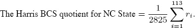
• If the Harris Interactive College Football Poll has 113 voting members for a given season, then the highest total rating that a team can achieve is 113 × 25 = 2, 825, which is attained if and only if all 113 members give that team a rating of r = 25, or equivalently, they all rank that team as #1. Similarly, the lowest total rating that a team can have is 113, obtained when each member assigns a rating of r = 1 to that team (i.e., everyone ranks the team #25). So, if ri is the Harris rating given to a team (say NC State) by the ith voter, then
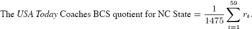
• If the USA Today Coaches Poll has 59 voting members for the same season, then the highest possible total rating is 59 × 25 = 1, 475. Consequently, if ri is the USA Today Coaches rating given to NC State by the ith voter, then
• Each of the six computer models provides numerical ratings for their top 25 teams just as the humans do—i.e., r = 25 for the highest ranked team, r = 24 for the second ranked team, etc. However, before computing the total sum of ratings for each team, the highest and lowest ratings for each team are dropped. Consequently, each team has only four computer ratings. These four ratings are summed to provide the total rating for each team. Thus the highest total computer rating that can be achieved is 4 × 25 = 100. For example, if the ratings for NC State from the six computer models are ordered as r1 ≥ r2 ≥ r3 ≥ r4 ≥ r5 ≥ r6, then
![]()
Putting It All Together. The BCS ratings and rankings at the end of each polling period are determined simply by adding together the BCS quotients defined above. While it makes no difference in the rankings, the average of the three BCS quotients is sometimes published instead of the sum of the BCS quotients because the average forces all final ratings to be in the interval (0, 1]. In other words,
![]()
The Recent BCS Computer Models. The computer models that have recently been used for the BCS computer rankings include those by the people listed below. However, the specifics of their methods are generally not available. Many developers do not want the details of their secret potions completely revealed, so they only hint at what they do.
1. Jeff Anderson and Chris Hester (www.andersonsports.com) give very little in the way of details other than to say that they reward teams for beating quality opponents, that they do not consider the margin of victory, and that their ratings depend not only on win-loss records but also on conference strength.
2. Richard Billingsley (www.cfrc.com) divulges nothing. It is theorized by others that the main components in his formula are win-loss records, opponents’ strength based on their records, ratings, and ranks (with a strong emphasis on most recent performances), and minor considerations for the site of the game and defensive performance.
3. Wesley Colley’s (www.colleyrankings.com) techniques are detailed in Chapter 3 on page 21.
4. Kenneth Massey’s early techniques are described on page 9, but he suggests that he now uses more refined (but not completely specified) methods—see masseyratings.com.
5. Jeff Sagarin (www.usatoday.com/sports/sagarin.htm) says that his model primarily utilizes the Elo system that is described in detail in Chapter 5 on page 53.
6. Peter Wolfe (prwolfe.bol.ucla.edu/cfootball/ratings.htm) states that his method is adapted from methods of Bradley and Terry in [13]. He says that it is a maximum likelihood scheme in which team i is assigned a rating value πi that is used in predicting the expected result when team i meets team j, with the likelihood of i beating j given by πi/(πi + πj). The probability P of all the results happening as they actually did is the product of multiplying together all the individual probabilities derived from each game. The rating values are chosen in such a way that the value of P is maximized. A similar technique is discussed by James Keener in [42].
ASIDE: No Wiggle Room Allowed
The BCS ratings narrow the competitors in the NCAA Division I Football Bowl Subdivision (or FBS—formerly Division I-A) to two teams that compete in the “BCS National Championship Game.” Voting members from the American Football Coaches Association are contractually obligated to vote the winner of this game as the “BCS National Champion.” Moreover, a contract signed by each conference requires them to recognize the winner of this game as the “official and only champion,” thus eliminating the possibility of multiple champions being crowned by the competing rating entities.
ASIDE: The Notre Dame Rule
The BCS ratings are used to determine which schools are given berths in post-season bowl games, but the ratings are tempered by a complicated set of tangled rules designed to protect various athletic conferences and historically powerful programs. Perhaps the most bizarre example is the “Notre Dame rule” that gives Notre Dame an automatic berth in the bowl games if it finishes in the top eight. And it get stranger. Notre Dame is also guaranteed a separate and unique payment reported to be 1/66th of the net BCS bowl revenues—regardless of their win-loss record for the season and regardless of whether or not they qualify for a bowl game! It was reported that the Fighting Irish were paid approximately $1,700,000 in 2009, a season in which they had only a 6-6 record and fired their coach, Charlie Weis. It has been estimated that if they had made a bowl game, then they would have been paid about $6,000,000.
The Notre Dame rule is an ongoing controversy. The exclusion of almost half the teams in the FBS from any realistic opportunities to win or compete for the BCS Championship while giving Notre Dame unique advantages and opportunities sticks in the craw of many fans.
ASIDE: Obama and the Department Of Justice
During his 2008 presidential campaign, then President-elect Obama appeared on Monday Night Football. ESPN sportscaster Chris Berman asked him to describe the one thing about sports that he would change, and Obama mentioned his disgust with using the BCS rating system to determine bowl-game participants. Instead, like many fans, he favored an eightteam playoff to determine the winner of the national title. Many fans wish the president would simply sign this suggestion into law.
In 2009 Senator Orrin Hatch of Utah asked the U.S. Justice Department to review the legality of the BCS for possible violations to antitrust laws. Hatch was motivated by the fact that the University of Utah had been undefeated but was denied a chance to play in the 2008 title game due to the peculiarities of the BCS system. Hatch and others cite antitrust issues that are at the heart of the “tremendous inequities,” citing the BCS’s favoritism of some conferences. For instance, under BCS rules, the champions of six conferences have automatic bids to play in the top-tier bowl games.
Atlantic Coast Conference |
→ |
Orange Bowl |
Big 12 Conference |
→ |
Fiesta Bowl |
Big East Conference |
→ |
No specific BCS Bowl |
Big Ten Conference |
→ |
Rose Bowl |
Pacific-12 Conference |
→ |
Rose Bowl |
Southeastern Conference |
→ |
Sugar Bowl |
In addition, these six conferences receive more money for these appearances than other conferences. However, conference alignments are currently in a state of flux, so several changes may have occurred by the time you read this.
As of May 2011, the BCS was put on notice that they are being scrutinized by the U. S. Department of Justice. Assistant Attorney General Christine Varney, the department’s antitrust division leader, reportedly sent a two-page letter to Mark Emmert (NCAA president at the time) stating that, “Serious questions continue to arise suggesting that the current Bowl Championship Series (BCS) system may not be conducted consistent with the competition principles expressed in federal antitrust laws.”