Chapter Six

The Markov Method

This new method for ranking sports teams invokes an old technique from A. A. Markov, and thus, we call it the Markov method.¹ In 1906 Markov invented his chains, which were later labeled as Markov chains, to describe stochastic processes. While Markov first applied his technique to linguistically analyze the sequence of vowels and consonants in Pushkin’s poem Eugene Onegin, his chains have found a plethora of applications since [8, 80]. Very recently graduate students of our respective universities, Anjela Govan (Ph.D. North Carolina State University, 2008) [34] and Luke Ingram (M.S., College of Charleston, 2007) [41] used Markov chains to successfully rank NFL football and NCAA basketball teams respectively.

The Markov Method

There are many measures by which teams can cast votes. Perhaps the simplest voting method uses wins and losses. A losing team casts a vote for each team that beats it. A more advanced model considers game scores. In this case, the losing team casts a number of votes equal to the margin of victory in its matchup with a stronger opponent. An even more advanced model lets both teams cast votes equal to the number of points given up in the matchup. At the end, the team receiving the greatest number of votes from quality teams earns the highest ranking. This idea is actually an adaptation of the famous PageRank algorithm used by Google to rank webpages [49]. The number of modeling tweaks is nearly endless as the discussion on page 71 shows. However, before jumping to enhancements, let’s go directly to our running example.

Voting with Losses

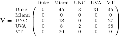
The voting matrix V that uses only win-loss data appears below.

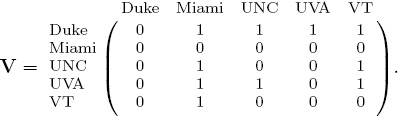
Because Duke lost to all its opponents, it casts votes of equal weight for each team. In order to tease a ranking vector from this voting matrix we create a (nearly) stochastic matrix N by normalizing the rows of V.

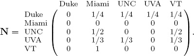
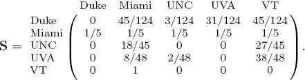
N is substochastic at this point because Miami is an undefeated team. This is akin to the well-known dangling node problem in the field of webpage ranking [49]. The solution there, which we borrow here, is to replace all 0^T rows with 1/n e^T so that N becomes a stochastic matrix S.

While dangling nodes (a webpage with no outlinks) are prevalent in the web context [51, 26], they are much less common over the course of a full sports season. Nevertheless, there are several other options for handling undefeated teams. Consequently, we devote the discussion on page 73 to the presentation of a few alternatives to the uniform row option used above.

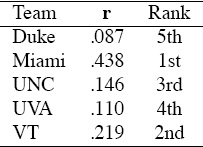
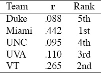
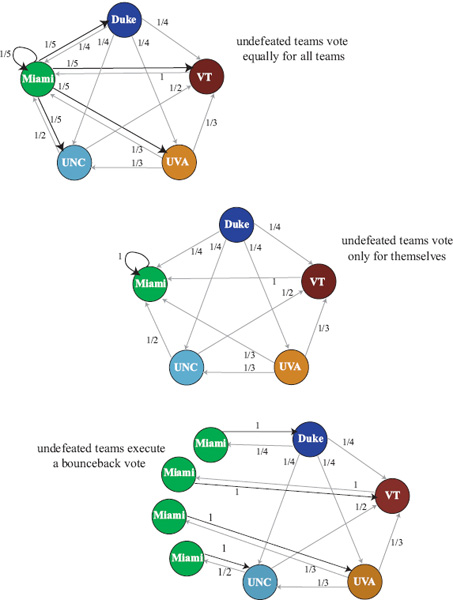
Again in analogy with the webpage PageRank algorithm we compute the stationary vector of this stochastic matrix. The stationary vector r is the dominant eigenvector of S and solves the eigensystem Sr = r [54]. The following short story explains the use of the stationary vector as a means for ranking teams. The main character of the story is a fair weather fan who constantly changes his or her support to follow the current best team. The matrix S can be represented with the graph in Figure 6.1. The fair weather fan starts at any node in this network and randomly chooses his next team to support based on the links leaving his current team. For example, if this fan starts at UNC and asks UNC, “who is the best team?”, UNC will answer “Miami or VT, since they both beat us.” The fan flips a coin and suppose he ends up at VT and asks the same question. This time VT answers that Miami is the best team and so he jumps on the Miami bandwagon. Once arriving at the Miami camp he asks his question again. Yet because Miami is undefeated he jumps to any team at random. (This is due to the addition of the 1/5 e^T row, but there are several other clever strategies for handling undefeated teams that still create a Markov chain with nice convergence properties. See page 73.) If the fair weather fan does this continually and we monitor the proportion of time he visits each team, we will have a measure of the importance of each team. The team that the fair weather fan visits most often is the highest ranked team because the fan kept getting referred there by other strong teams. Mathematically, the fair weather fan takes a random walk on a graph defined by a Markov chain, and the long-run proportion of the time he spends in the states of the chain is precisely the stationary vector or dominant eigenvector of the chain. For the five-team example, the stationary rating vector r of S and its corresponding ranking are in Table 6.1.

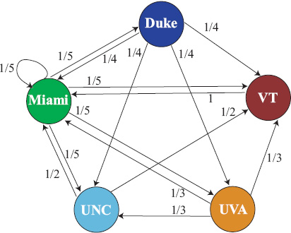
Figure 6.1 Fair weather fan takes a random walk on this Markov graph

Table 6.1 Markov:Losses rating results for the 5-team example

Losers Vote with Point Differentials

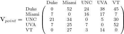
Of course, teams may prefer to cast more than one vote for opponents. Continuing with the fair weather fan story, UNC might like to cast more votes for VT than Miami since VT beat them by 27 points while Miami only beat them by 18. In this more advanced model, the voting and stochastic matrices are

and

This model produces the ratings and rankings listed in Table 6.2. Voting with point differentials results in a slightly different ranking yet significantly different ratings from the elementary voting model. Such differences may become important if one wants to go beyond predicting winners to predict point spreads.

Table 6.2 Markov:Point Differentials rating results for the 5-team example

When two teams faced each other more than once in a season, the modeler has a choice for the entries in the voting matrix. The entry can represent either the cumulative or the average point differential between the two teams in all matchups that season.

Winners and Losers Vote with Points

In a yet more advanced model, we let both the winning and losing teams vote with the number of points given up. This model uses the complete point score information. In this case, the V and S matrices (which we now label V_point and S_point to distinguish them from the matrices on page 72) are

and

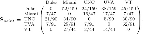
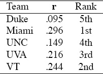
Notice that this formulation of S has the added benefit of making the problem of undefeated teams obsolete. A zero row appears in the matrix only in the unlikely event that a team held all its opponents to scoreless games. The rating and ranking vectors for this model appear in Table 6.3.

Table 6.3 Markov:Winning and Losing Points rating results for the 5-team example

Beyond Game Scores

Sports fans know that game scores are but one of many statistics associated with a contest. For instance, in football, statistics are collected on yards gained, number of turnovers, time of possession, number of rushing yards, number of passing yards, ad nauseam. While points certainly have a direct correlation with game outcomes, this is ultimately not the only thing one may want to predict (think: point spread predictions). Naturally, a model that also incorporates these additional statistics is a more complete model. With the Markov model, it is particularly easy to incorporate additional statistics by creating a matrix for each statistic. For instance, using the yardage information from Table 6.4 below, we build a voting matrix for yardage whereby teams cast votes using the number of yards given up.

Table 6.4 Total yardage data for the 5-team example

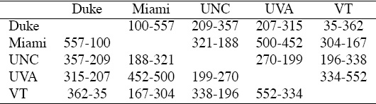
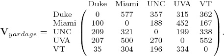
The (Duke, Miami) element of 577 means that Duke allowed Miami to gain 577 yards against them and thus Duke casts votes for Miami relative to this large number. Row normalizing produces the stochastic matrix S_yardage below.

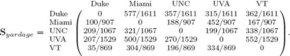
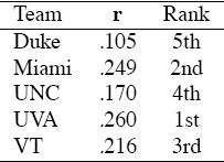
The rating and ranking vectors produced by S_yardage appear in Table 6.5.

Table 6.5 Markov:Yardage rating results for the 5-team example

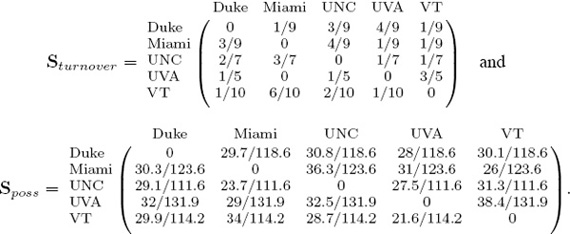
Of course, there’s nothing special about point or yardage information—any statistical information can be incorporated. The key is to simply remember the voting analogy. Thus, in a similar fashion the S_turnover and S_poss matrices are

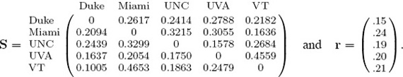
The next step is to combine the stochastic matrices for each individual statistic into a single matrix S that incorporates several statistics simultaneously. As usual, there are a number of ways of doing this. For instance, one can build the lone global S as a convex combination of the individual stochastic matrices, S_point, S_yardage, S_turnover, and S_poss so that

S = α₁S_point + α₂S_yardage + α₃S_turnover + α₄S_poss,

where α₁, α₂, α₃, α₄ ≥ 0 and α₁ + α₂ + α₃ + α₄ = 1. The use of the convex combination guarantees that S is stochastic, which is important for the existence of the rating vector. The weights α_i can be cleverly assigned based on information from sports analysts. However, to demonstrate the model now, we use the simple assignment α₁ = α₂ = α₃ = α₄ = 1/4, which means

The beauty of the Markov model is its flexibility and ability for almost endless tuning. Nearly any piece of statistical information (home-field advantage, weather, injuries, etc.) can be added to the model. Of course, the art lies in the tuning of the α_i parameters.

Handling Undefeated Teams

Some of the methods for filling in entries of the Markov data that were described earlier in this chapter make it very likely to encounter a row of all zeros, which causes the Markov matrix to be substochastic. This substochasticity causes a problem for the Markov model, which requires a row stochastic matrix in order to create a ranking vector. In the example on page 68, we handled the undefeated team of Miami with a standard trick from webpage ranking—replace all 0^T rows with 1/n e^T. While this mathematically solves the problem and creates a stochastic matrix, there are other ways to handle undefeated teams that may make more sense in the sports setting.

For instance, rather than forcing the best team to cast an equal number of votes for each team, including itself, why not let the best team vote only for itself. In this case, for each undefeated team i, replace the 0^T row with , which is a row vector representing the i^th row of the identity matrix. Now the data creates a stochastic matrix and hence a Markov chain. However, this fix creates another problem. In fact, this is a potential problem that pertains to the reducibility of the matrix for all Markov models, though it is a certainty in this case. In order for the stationary vector to exist and be unique, the Markov chain must be irreducible (and also aperiodic, which is nearly always satisfied) [54]. An irreducible chain is one in which there is a path from every team to every other team. When undefeated teams vote only for themselves, the chain is reducible as these teams become absorbing states of the chain. In other words, the fair weather fan who takes a random walk on the graph will eventually get stuck at an undefeated team. Here again we employ a trick from webpage ranking and simply add a so-called teleportation matrix E to the stochasticized voting matrix S [49]. Thus, for 0 ≤ β ≤ 1, the Markov matrix is

= βS + (1 − β)/nE,

where E is the matrix of all ones and n is the number of teams. Now is irreducible as every team is directly connected to every other team with at least some small probability, and the stationary vector of exists and is unique. This rating vector depends on the choice of the scalar β. Generally the higher β is, the truer the model stays to the original data. When the data pertains to the Web, β = .85 is a commonly cited measure [15]. Yet for sports data, a much lower β is more appropriate. Experiments have shown β = .6 works well for NFL data [34] and β = .5 for NCAA basketball [41]. Regardless, the choice for β seems application, data, sport, and even season-specific.

Another technique for handling undefeated teams is to send the fair weather fan back to the team he just came from, where he can then continue his random walk. This bounce-back idea has been implemented successfully in the webpage ranking context [26, 53, 49, 77] where it models nicely the natural reaction of using the BACK button in a browser. While this bounce-back idea is arguably less pertinent in the sports ranking context, it may, nevertheless, be worth exploring. The illustration below summarizes the three methods for handling undefeated teams.

Summary of the Markov Rating Method

The shaded box below assembles the labeling conventions we have adopted to describe our Markov method for ranking sports teams.

Since most mathematical software programs, such as MATLAB and Mathematica, have built-in functions for computing eigenvectors, the instructions for the Markov method are compact.

We close this section with a list of properties of Markov ratings.

• In a very natural way the Markov model melds many game statistics together.

• The rating vector r > 0 has a nice interpretation as the long-run proportion of time that the fair weather fan (who is taking a random walk on the voting graph) spends with any particular team.

• The Markov method is related to the famous PageRank method for ranking webpages [14].

• Undefeated teams manifest as a row of zeros in the Markov matrix, which makes the matrix substochastic and causes problems for the method. In order to produce a ranking vector, each substochastic row must be forced to be stochastic somehow. The discussion on page 73 outlines several methods for doing this and forces undefeated teams to vote.

• The stationary vector of the Markov method has been shown, like PageRank, to follow a power law distribution. This means that a few teams receive most of the rating, while the great majority of teams must share the remainder of the miniscule leftover rating. One consequence of this is that the Markov method is extremely sensitive to small changes in the input data, particularly when those changes involve low-ranking teams in the tail of the power law distribution. In the sports context, this means that upsets can have a dramatic and sometimes bizarre effect on the rankings. See [21] for a detailed account on this phenomenon.

Connection between the Markov and Massey Methods

While the Markov and Massey methods seem to have little in common, a graphical representation reveals an interesting connection. As pointed out earlier in this chapter, there are several ways to vote in the Markov method. Because the Massey method is built around point differentials, the Markov method that votes with point differentials is most closely connected to the Massey method. Consider Figure 6.2, which depicts the Markov graph associated with the point differential voting matrix V of page 70. This graph actually holds precisely the same information used by the Massey method. Recall the fundamental equation of the Massey method, which for a game k between teams i and j creates a linear equation of the form r_i − r_j = y_k, meaning that team i beat team j by y_k points in that matchup. Thus for our five team example, since VT beat UNC by 27 points, Massey creates the equation r_VT − r_UNC = 27. If we create a graph with this point differential information, we have the graph of Figure 6.3, which is simply the transpose of the Markov graph. Both graphs use point differentials to weight the links but the directionality of the links is different. In the Massey graph, the direction of the link indicates dominance whereas it signifies weakness in the Markov graph.

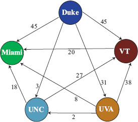
Figure 6.2 Markov graph of point differential voting matrix

Though the two graphs are essentially the same, the two methods are quite different in philosophy. Given the weights from the links, both methods aim to find weights for the nodes. The Markov method finds such node weights with a random walk. Recall the fair weather fan who takes a random walk on this graph (or more precisely, the stochasticized version of this graph). The long-run proportion of time the fair weather fan spends at any node i is its node weight r_i. On the other hand, the Massey method finds these node weights with a fitting technique. That is, it finds the node weights r_i that best fit the given link weights. Perhaps the following metaphors are helpful.

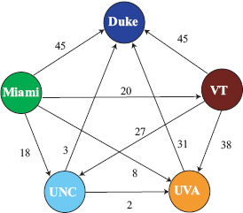
Figure 6.3 Massey graph for the same five team example as Figure 6.2

ASIDE: PageRank and the Random Surfer

ASIDE: Ranking U.S. Colleges

The controversy surrounding the US News college rankings prompted us to explore how these rankings are created. First, the participating colleges and universities are placed into particular categories based on the Carnegie classifications published annually by the Carnegie Foundation for the Advancement of Teaching. For example, the Carnegie classification of Research I applies to all Ph.D.-granting institutions of a certain size. There are similar classifications for Master’s I and Master’s II schools. Schools are only compared with those in the same Carnegie category. Data are collected about the schools using forms from the Common Data Set developed by US News, Peterson’s, and The College Board. Roughly 75% of this information is numerical data, which covers seven major topics: peer assessment, retention and graduation of students, faculty resources, student selectivity, financial resources, alumni giving, and graduation rate. The remaining 25% comes from the subjective ratings of college presidents and deans who are queried about their peer institutions, i.e., schools in their Carnegie classification. US News combines this numerical and subjective data using a simple weighted mean whose weights are determined by educational research analysts.

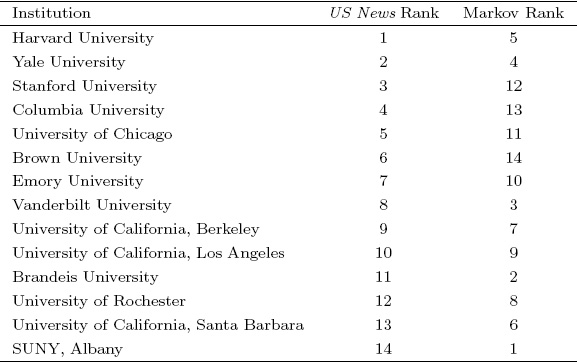
Surprised by the simplicity of the ranking method incorporated by US News, we were tempted to compare the US News ranking with a more sophisticated ranking method such as the Markov method. For demonstration purposes, we decided to rank fourteen schools that all had the same Carnegie classification. We created a single Markov matrix built from seven matrices based on the following seven factors: number of degrees of study, average institutional financial aid, tuition price, faculty to student ratio, acceptance rate, freshman retention rate, and graduation rate.

Table 6.6 shows both the US News ranking (from August 2007) and the Markov ranking for these fourteen schools. Clearly, the two rankings are quite different. Notice, for instance, that SUNY went from last place among its peers in the US News ranking to first place in the Markov ranking. Since it is hard to say which ranking is better, our point here is simply that different methods can produce vastly different rankings. And when so much is riding on a ranking (i.e., a school’s reputation, and thus, revenue), a sophisticated rigorous method seems preferable.

Table 6.6 College rankings by US News and Markov methods

¹There are at least two other existing sports ranking models that are based on Markov chains. One is the product of Peter Mucha and his colleagues and is known as the Random Walker rating method [17]. The other is the work of Joel Sokol and Paul Kvam and is called LRMC [48].