Chapter Five

Elo’s System

Árpád Élö (1903–1992) was a Hungarian-born physics professor at Marquette University in Milwaukee, Wisconsin. In addition, he was an avid (and excellent) chess player, and this led him to create an effective method to rate and rank chess players. His system was approved by the United States Chess Federation (USCF) in 1960, and by Fédération Internationale des Échecs (the World Chess Federation, or FIDE) in 1970. Elo’s idea eventually became popular outside of the chess world, and it has been modified, extended, and adapted to rate other sports and competitive situations. The premise that Elo used was that each chess player’s performance is a normally distributed random variable X whose mean μ can change only slowly with time. In other words, while a player might perform somewhat better or worse from one game to the next, μ is essentially constant in the short-run, and it takes a long time for μ to change.

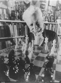
Arpad Elo

As a consequence, Elo reasoned that once a rating for a player becomes established, then the only thing that can change the rating is the degree to which the player is performing above or below his mean.¹ He proposed a simple linear adjustment that is proportional to the player’s deviation from his mean. More specifically, if a player’s recent performance (or score²) is S, then his old rating r(old) is updated to become his new rating by setting

where K is a constant—Elo originally set K = 10. As more chess statistics became available it was discovered that chess performance is generally not normally distributed, so both the USCF and FIDE replaced the original Elo assumption by one that postulates the expected scoring difference between two players is a logistic function of the difference in their ratings (this is described in detail on page 54). This alteration affects both μ and K in (5.1), but the ratings are still referred to as “Elo ratings.”

In 1997 Bob Runyan adapted the Elo system to rate international football (what Americans call soccer), and at some point Jeff Sagarin, who has been providing sports ratings for USA Today since 1985, began adapting Elo’s system for American football.

In its present form, the Elo system works like this. You must start with some initial set of ratings (see page 56) for each competitor—to think beyond chess, consider competitors as being teams. Each time teams i and j play against each other, their respective prior ratings r_i(old) and r_j(old) are updated to become r_i(new) and r_j(new) by using formulas similar to (5.1). But now everything is going to be considered on a relative basis in the sense that S in (5.1) becomes

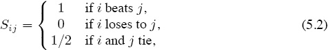
and μ becomes

μ_ij = the number of points that team i is expected to score against team j.

The new assumption is that μ_ij is a logistic function of the difference in ratings

d_ij = r_i(old) − r_j(old)

prior to teams i and j playing a game against each other. The standard logistic function is defined to be f(x) = 1/(1 + e^−x), but chess ratings employ the base-ten version

The functions f(x) and L(x) are qualitatively the same because 10^−x = e^{−x(ln 10)}, and their graphs each have the following characteristic s-shape.

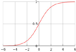
Figure 5.1 Graph of a logistic function

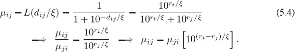
The precise definition of μ_ij for Elo chess ratings is

so the respective formulas for updating ratings of teams (or players) i and j are as follows.

Elegant Wisdom

The simple elegance of the Elo formula belies its wisdom in the sense that Elo inherently rewards a weaker player for defeating a stronger player to greater degree than it rewards a stronger player for beating a weak opponent. For example, if an average chess player’s rating is 1500 while that of a stronger player is 1900, then

but

Therefore, the reward to the average player for beating the stronger player is

r_avg(new) − r_avg(old) = K(S_avg,str − μ_avg,str) = K(1 − .09) = .91K,

whereas if the stronger player defeats the average player, then the reward is only

r_str(new) − r_str(old) = K(S_str,avg − μ_str,avg) = K(1 − .91) = .09K.

The K-Factor

The “K-factor,” as it is know in chess circles, is still a topic of discussion, and different values are used by different chess groups. Its purpose is to properly balance the deviation between actual and expected scores against prior ratings.

If K is too large, then too much weight is given to the difference between actual and expected scores, and this results in too much volatility in the ratings—e.g., a big K means that playing only a little above expectations can generate a big change in the ratings. On the other hand, if K is too small, then Elo’s formulas lose their ability to account for improving or deteriorating play, and the ratings become too stagnant—e.g., a small K means that even a significant improvement in one’s play cannot generate much of a change in the ratings.

Chess:  The K-factor for chess is often allowed to change with the level of competition. For example, FIDE sets

K = 25 for new players until 30 recognized games have been completed;
K = 15 for players with > 30 games whose rating has never exceeded 2400;
K = 10 for players having reached at least 2400 at some point in the past.

At the time of this writing FIDE is considering changing these respective K-factors to 30, 30, and 20.

Soccer: Some raters of soccer (international football) allow the value of K to increase with the importance of the game. For example, it is not uncommon to see Internet sites report that the following K values are being used.

K = 60 for World Cup finals;
K = 50 for continental championships and intercontinental tournaments;
K = 40 for World Cup qualifiers and major tournaments;
K = 30 for all other tournaments;
K = 20 for friendly matches.

The K-factor is one of those things that makes building rating systems enjoyable because it allows each rater the freedom to customize his/her system to conform to the specific competition being rated and to add their own personal touch.

The Logistic Parameter ξ

The parameter ξ = 400 in the logistic function (5.3) comes from the chess world, and it affects the spread of the ratings. To see what this means in terms of comparing two chess players with respective ratings r_i and r_j, do a bit of algebra to observe that

Since μ_ij is the number points that player i is expected to score against player j, this means that if r_i−r_j = 400, then player i is expected to be ten times better than player j. In general, for every 400 rating points of advantage that player i has over player j, the probability of player i beating player j is expected to be ten times greater than the probability of player j beating player i.

Moving beyond chess, the same analysis as that used above shows that replacing 400 in (5.3) by any value ξ > 0 yields

Now, for every ξ rating points of advantage that team i has over team j, the probability of team i beating team j is expected to be ten times greater than the probability of team j beating team i. Fiddling with ξ is yet another way to tune the system to make it optimal for your particular needs.

Constant Sums

When scores S_ij depend only on wins, loses, and ties as described in (5.2) for chess, then S_ij + S_ji = 1, and (as shown below) this will force the Elo ratings to always sum to a constant value, regardless of how many times ratings are updated. This constant-sum feature also holds for competitions in which S_ij depends on numbers of points scored provided S_ij + S_ji = 1. Below is the formal statement and proof.

Proof. Notice that regardless of the value of the logistic parameter ξ, equation (5.4) ensures that

μ_ij + μ_ji = 1.

This together with S_ij + S_ji = 1 means that after a game between teams i and j, the respective updates (from page 54) to the old ratings r_i(old) and r_j(old) are K(S_ij − μ_ij) and K(S_ji − μ_ji), so

Therefore,

Caution! Equation (5.5) says that the change in the rating for team i is just the negative of that for team j, but this does not mean that r_i(new) + r_j(new) = 0.

Elo in the NFL

To see how Elo performs on something other than chess we implemented the basic Elo scheme that depends only on wins and loses to rate and rank NFL teams for the 2009–2010 season. We considered all of the 267 regular-season and playoff games, and we used the same ordering of the teams as shown in the table on page 42.

While we could have used standings from prior years or from preseason games, we started everything off on an equal footing by setting all initial ratings to zero. Consequently the ratings at any point during the season as well as the final ratings sum to zero, and thus their mean value is zero.

Together with the win-lose scoring rule (5.2) on page 54, we used a K-factor of K = 32 (a value used on several Internet gaming sites and in line with those of the chess community), but we increased the logistic factor from 400 to ξ = 1000 to provide a better spread in the final ratings. The final rankings are not sensitivie to the value of ξ, and our increase in ξ did not significantly alter the final rankings, which are shown below.

NFL 2009–2010 Elo rankings based only on wins & loses with ξ = 1000 and K = 32

Since these Elo ratings are compiled strictly on the basis of wins and loses, it would be surprising if they were not well correlated with the win percentages reported in (4.18) on page 46. Indeed, the correlation coefficient (4.20) is R_rw = .9921. Proceeding with linear regression as we did for the Keener ratings on pages 47 and 48 produces

Est Win% for team i = .5 + .0022268 r_i,

which in turn yields

MAD = .017958 and MSE = .0006.

While these are good results, it is not clear that they are significant because in essence they boil down to using win-lose information to estimate win percentages.

A more interesting question is, how well does Elo predict who wins in the NFL?

Hindsight Accuracy

While it is not surprising that Elo is good at estimating win percentages, it is not clear what to expect if we take the final Elo ratings back in time as described on page 48 to predict in hindsight who wins each game. Looking back at the winners of all of the 267 NFL games during 2009–2010 and comparing these with what Elo predicts—i.e., the higher final rated team is predicted to win—we see that Elo picks 201 game correctly, so

Elo Hindsight Accuracy = 75.3%.

While it seems reasonable to add a home-field-advantage factor to each of the ratings for the home team in order to predict winners, incorporating a home-field-advantage factor does not improve the hindsight accuracy for the case at hand.

As mentioned in the Keener discussion on page 48, the “hindsight is 20-20” cliché is not valid for rating systems—even good ones are not going to predict all games correctly in hindsight. The Elo hindsight accuracy of 75.3% is very good—see the table of comparisons on page 123.

Foresight Accuracy

A more severe test of a ranking system is how well the vector r(j) of ratings that is computed after game j can predict the winner in game j + 1. Of course, we should expect this foresight accuracy to be less than the hindsight accuracy because hindsight gets to use complete knowledge of all games played while foresight is only allowed to use information prior to the game currently being analyzed.

A home-field-advantage factor matters much more in Elo foresight accuracy than in hindsight accuracy because if all initial ratings are equal (as they are in our example), then in the beginning, before there is enough competition to change each team’s ratings, home-field consideration is the only factor that Elo can use to draw a distinction between two teams. When a home-field advantage factor of H = 15 is added to the ratings of the home team when making foresight predictions from the game-by-game ratings computed with ξ = 1000 and K = 32, Elo correctly predicts the winner in 166 out of 267 games, so

Elo Foresight Accuracy = 62.2%.

Incorporating Game Scores

Instead of building ratings based just on wins and loses, let’s jazz Elo up a bit by using the number of points P_ij that team i scores against team j in each game. But rather than using raw scores directly, apply the logic that led to (4.2) on page 31 to redefine the “score” that team i makes against team j to be

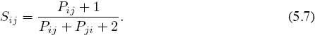
In addition to having 0 < S_ij < 1, this definition ensures that S_ij + S_ji = 1 so that S_ij can be interpreted as the probability that team i beats team j (assuming that ties are excluded). Moreover, if all initial ratings are zero (as they are in the previous example), then the discussion on page 56 means that as the Elo ratings change throughout the season, they must always sum to zero and the mean rating is always zero.

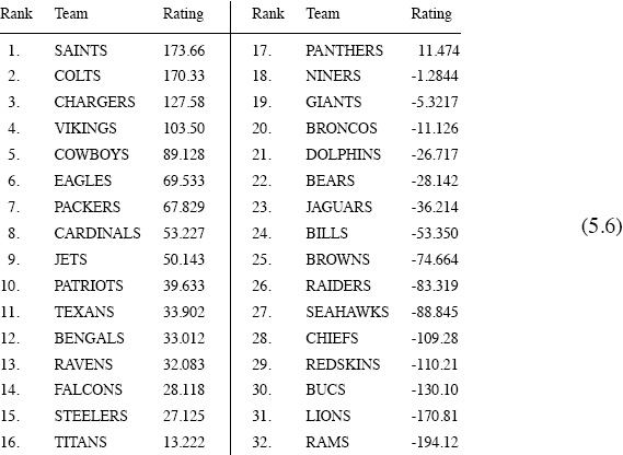
When the parameters ξ = 1000 and K = 32 (the same as those from the basic win-lose Elo scheme) are used with the scores in (5.7), Elo produces the following modified ratings and rankings.

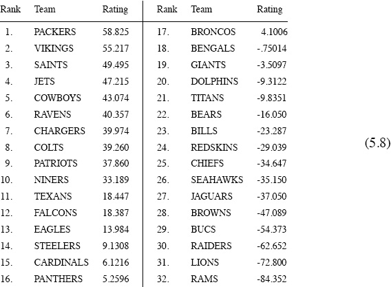
NFL 2009–2010 Elo rankings using scores with ξ = 1000 and K = 32

Hindsight and Foresight with ξ = 1000, K = 32, H = 15

The ratings in (5.8) produce both hindsight and foresight predictions in a manner similar to the earlier description. But unlike the hindsight predictions produced by considering only wins and losses, the home-field-advantage factor H matters when scores are being considered. If H = 15 (empirically determined) is used for both hindsight and foresight predictions, then the ratings in (5.8) correctly predict

194 games (or 72.7%) in hindsight, and 175 games (or 65.5%) in foresight.

Using Variable K-Factors with NFL Scores

The ratings in (5.8) suffer from the defect that they are produced under the assumption that all games are equally important—i.e., the K-factor was the same for all games. However, it can be argued that NFL playoff games should be more important than regular-season games in determining final rankings. Furthermore, there is trend in the NFL for stronger teams to either rest or outright refuse to play their key players to protect them from injuries during the final one or two games of the regular season—this certainly occurred in the final two weeks of the 2009–2010 season.

Consequently, the better teams play below their true scoring ability during this time while their opponents appear to Elo to be stronger than they really are. This suggests that variable K-factors should be used to account for these situations.

Let’s try to fix this by setting (rather arbitrarily)

K = 32 for the first 15 weeks;
K = 16 for the final 2 weeks;
K = 64 for all playoff games.

Doing so (but keeping ξ = 1000) changes the Elo ratings and rankings to become those shown below in (5.9).

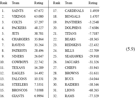
NFL 2009–2010 Elo rankings using scores with ξ = 1000 and K = 32, 16, 64

As far as final rankings are concerned, these in (5.9) look better than those in (5.8) because (5.9) more accurately reflects what actually happened when all the dust had settled. The SAINTS ended up being ranked #1 in (5.9), and, as you can see from the playoff results in Figure 5.2, the SAINTS won the Super Bowl. Furthermore, the VIKINGS gave the SAINTS a greater challenge than the COLTS did during the playoffs, and this showed up in the final ratings and rankings in (5.9).

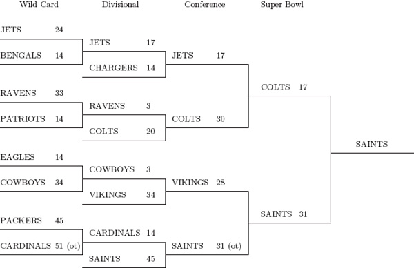
Figure 5.2 NFL 2009–2010 playoff results

Hindsight and Foresight Using Scores and Variable K-Factors

The ratings in (5.9) better reflect the results of the playoffs than those in (5.8), but the ability of (5.9) to predict winners is only slightly better than that of (5.8). Changing the K-factor from a constant K = 32 to a variable K = 32, 16, 64 changes the value of the ratings, so the home-field-advantage factor H must also be changed—what works best is to use H = 0 for hindsight predictions and H = 9.5 for foresight predictions. With these values the variable-K Elo system correctly predicts

194 games (or 72.7%) in hindsight, and 176 games (or 65.9%) in foresight.

Game-by-Game Analysis

Tracking individual team ratings on a game-by-game basis throughout the season provides a sense of overall strength that might not be apparent in the final ratings. For example, when an Elo system that gives more weight to playoff games and discounts the “end-of-season throw-away games” is used (as was done in (5.9)), it is possible that a team may have a higher final ranking than it deserves just because it has a good playoff series. For example, consider the game-by-game ratings for the three highest ranked teams in (5.9). The following three graphs track the game-by-game ratings of the SAINTS vs. COLTS, the SAINTS vs. VIKINGS, and the COLTS vs. VIKINGS.

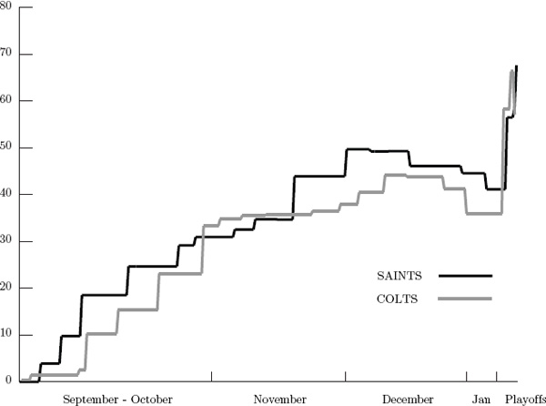
Game-by-game tracking of Elo ratings for SAINTS vs. COLTS

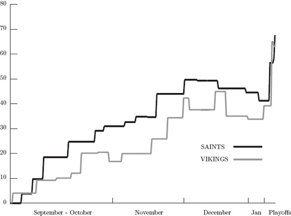
Game-by-game tracking of Elo ratings for SAINTS vs. VIKINGS

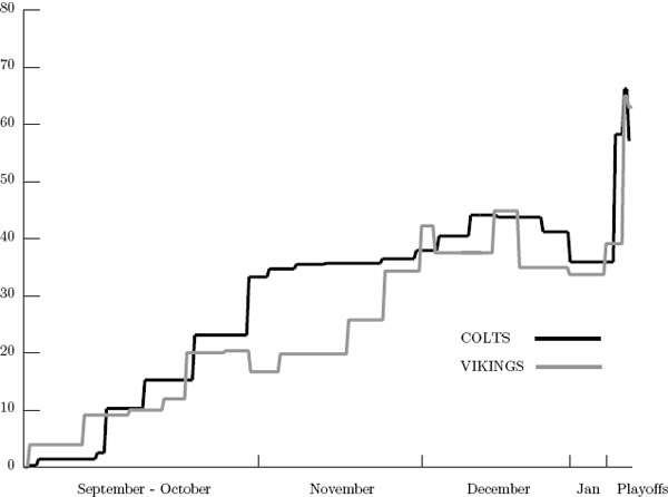
Game-by-game tracking of Elo ratings for COLTS vs. VIKINGS

Notice that the SAINTS are almost always above both the VIKINGS and the COLTS, so this clearly suggests that the SAINTS were the overall stronger team throughout the 2009–2010 season. But how do the COLTS and VIKINGS compare? If the ratings for each are integrated over the entire season (i.e., if the area under the graph of each team in the last graph above is computed), then the COLTS come out ahead of the VIKINGS. In other words, in spite of the fact that VIKINGS are ranked higher than the COLTS in the final ratings, this game-by-game analysis suggests that the COLTS were overall stronger than the VIKINGS across the whole season. As an unbiased fan who saw just about every game that both the COLTS and VIKINGS played during the 2009–2010 season (yes, I [C. M.] have the Sunday Ticket and a DVR), I tend to agree with this conclusion.

Conclusion

The Elo rating system is the epitome of simple elegance. In addition, it is adaptable to a wide range of applications. Its underlying ideas and principles might serve you well if you are trying to build a rating system from the ground up.

Regardless of whether or not there was an actual connection between Elo and Facebook, the following aside helps to underscore the adaptability of Elo’s rating system.

ASIDE: Elo, Hot Girls, and The Social Network

 

 

 

 

 

¹The assumption that performance is a normally distributed random variable and the idea of defining ratings based on deviations from the mean is found throughout the literature. The paper by Ashburn and Colvert [6] and its bibliography provides statistically inclined readers with information along these lines.

²In chess a win is given a score of 1 and a draw is given a score of 1/2. Performance might be measured by scores from a single match or by scores accumulated during a tournament.