
Chapter Four
Keener’s Method
James P. Keener proposed his rating method in a 1993 SIAM Review article [42]. Keener’s approach, like many others, utilizes nonnegative statistics that result from contests (games) between competitors (teams) to create a numerical rating for each team. In some circles these are called power ratings. Of course, once a numerical rating for each team is established, then ranking the teams in order of their ratings is a natural consequence.
Keener’s method is to relate the rating for a given team to the absolute strength of the team, which in turn depends on the relative strength of the team—i.e., the strength of the team relative to the strength of the teams that it has played against. This will become more clear as we proceed. Keener bases everything on the following two stipulations that govern the relationship between a team’s strength and its rating.
Strength and Rating Stipulations
1. The strength of a team should be gauged by its interactions with opponents together with the strength of these opponents.
2. The rating for each team in a given league should be uniformly proportional to the strength of the team. More specifically, if si and ri are the respective strength and rating values for team i, then there should be a proportionality constant λ such that si = λri, and λ must have the same value for each team in the league.
Selecting Strength Attributes
To turn the two rules above into a mechanism that can be used to compute a numerical rating for each team, let’s assign some variables to various quantities in question. First, settle on some attribute or statistic of the competition or sport under consideration that you think will be a good basis for making relative comparisons of team strength, and let
aij = the value of the statistic produced by team i when competing against team j.
For example one of the simplest statistics to consider is the number of times that team i has defeated team j during the current playing season. For ties, assign the participants a value of 1/2 for each time they have tied. In other words, if Wij is the number of times that team i has recently beaten team j, and if Tij is the number of times that teams i and j have tied, then you might set
![]()
If you think that a more relevant attribute that reflects team i’s power relative to that of team j is the number of points Sij that i scores against j, then you might define
aij = Sij.
If teams i and j play against each other more than once, then Sij is the cumulative number of points scored by i against j.
Rather than game scores or number of victories, you might choose to use other attributes of the competition. For example, if you are an old-school football fan who believes that the stronger football teams are those that excel in the running game, then you may want to set
aij = the number of rushing yards that team i accumulates against team j.
Similarly, a contemporary connoisseur of the NFL could be convinced that it’s all about passing, in which case
aij = the number of passing yards that team i gained against team j.
Regardless of what attribute you select to define your aij’s you will have to continually update them throughout the playing season (unless of course you are only evaluating the league after all competition is finished). But as you update your aij’s, you have to decide if the value of an attribute at the beginning of the season should have as much influence as its value near the end of the season—i.e., do you want to weight the aij’s as a function of time?
All of this flexibility allows for a lot of fiddling and tweaking, and this is what makes building rating and ranking models so much fun. As you can already begin to see, Keener’s method is particularly ripe with opportunities for tinkering, and even more such opportunities will emerge in what is to come.
Laplace’s Rule of Succession
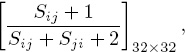
Regardless of the attribute that you select, the statistics concerning your attribute can rarely be used in their raw form to create a successful rating technique. For example, consider scores Sij. If teams i and j each have a weak defense but a good offense, then they are prone to rack up big scores against each other. On the other hand, if teams p and q each have a strong defense but a weak offense, then their games are likely to be low scoring. Consequently, the large Sij and Sji can have a disproportionate effect in any subsequent rating system compared to the small Spq and Sqp. When comparing teams i and j, it is better to take into account the total number of points scored by setting
![]()
Similar remarks hold for other attributes—e.g., rushing yards, passing yards, turnovers, etc.
Proportions aij generated by using ratios such as (4.1) may be better than using raw values, but, as Keener points out, we should really be using something like
![]()
The motivation for this is Laplace’s rule of succession [29], and the intuition is that if
![]()
and pij can be interpreted as the probability that team i will defeat team j in the future. If team i defeated team j by a cumulative score of X to 0 in past games where X > 0, then it might be reasonable to conclude that team i is somewhat better than team j (slightly better if X is small or much better if X is large). However, regardless of the value of X > 0, we have that
![]()
This suggests that it is impossible for team j to ever beat team i in the future, which is clearly unrealistic. On the other hand, if (4.2) is interpreted as the probability pij that team i will defeat team j in the future, then you can see from (4.2) that 0 < pij < 1, and if team i defeated team j by a cumulative score of X to 0 in the past, then
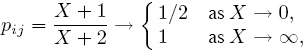
which is more reasonable than (4.3). Moreover, if Sij ≈ Sji and both are large, then pij ≈ 1/2, but as the difference Sij − Sji > 0 increases, pij gets closer to 1, which makes sense. Consequently, using (4.2) is preferred over (4.1).
To Skew or Not to Skew?
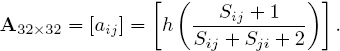
Skewing concerns the issue of how to compensate for the “just because we could” situation in which a stronger team mercilessly runs up the score against a weaker opponent to either enhance their own rating or perhaps to just “rub it in.” If (4.2) is used, then Keener suggests applying a nonlinear skewing function such as
![]()
to each of the aij’s to help mitigate differences at the upper and lower ends. In other words, replace aij by h(aij). The graph of h(x) is shown in Figure 4.1, and, as you can see, this function has the properties that h(0) = 0, h(1) = 1, and h(1/2) = 1/2. Using the h(aij)’s in place of the aij’s has the intended effect of somewhat moderating differences at the upper and lower ranges. Skewing with h(x) also introduces an artificial separation between two raw values near 1/2, which might be helpful in distinguishing between teams of nearly equal strength.
Once you have seen Keener’s skewing function in (4.4) and have played with it a bit, you should be able to construct many other skewing functions of your own. For example, you may want to customize your skewing function so that it is more or less exaggerated in its skewing ability than is h(x), or perhaps you need your function to affect the upper ranges of the aij’s differently than how it affects the lower ranges. The value of Keener’s skewing idea is its ability to allow you to “tune” your system to the particular competition being modeled. Skewing is yet another of the countless ways to fiddle with and tweak Keener’s technique.
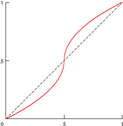
Figure 4.1 Graph of the skewing function h(x)
Skewing is not always needed. For example, skewing did not significantly affect the NFL rankings in the studies in [34, 35, 1]. This is probably due to the fact that the NFL was well balanced for the years under consideration, so the need for fine tuning was not so great. Of course, things are generally much different for NCAA sports or other competitions, so don’t discount Keener’s skewing idea.
Normalization
Having settled on the attribute that defines your nonnegative aij’s, and having decided whether or not you want to skew them by redefining aij ← h(aij), one last bit of massaging (or normalization) of the aij’s is required for situations in which not all teams play the same number of games. In such a case, make the replacement
![]()
To understand why this is necessary, suppose that you are using scores Sij to define your aij’s along the lines of (4.1) or (4.2). Teams playing more games than other teams have the possibility of producing more points, and thus inducing larger values of aij. This in turn will affect any measure of “strength” that is eventually derived from your aij’s. The same is true for statistics other than scores—e.g., if number of yards gained or number of passes completed is your statistic, then teams playing more games can accumulate higher values of these statistics, which in turn will affect any ratings that these statistics produce.
Caution! Skewing has a normalization effect, so if you are using a skewing function and there is not a large discrepancy in the number of games played, then (4.5) may not be necessary—you run the risk of “over normalizing” your data. Furthermore, different situations require different normalization strategies. Using (4.5) is the easiest thing to do and is a good place to start, but you may need to innovate and experiment with other strategies to obtain optimal results—yet another place for fiddling.
Chicken or Egg?
Once the aij’s are defined, skewed, and normalized, organize them into a square matrix
A = [aij]m×m, where m = the number of teams in the league.
Representing the data in such a way allows us to apply some extremely powerful ideas from matrix theory to quantify “strength” and to generate numerical ratings. While it is not apparent at this point, it will be necessary to make a subtle distinction between the “strength value” for each team and its “ratings value.” This will become more apparent in the sequel. In spite of the fact that the “strength value” and the “rating value” are not equal, they are of course related. This presents us with a chicken-or-egg situation because we would like to use the “rating values” to measure “strength values” but the “strength” of each team will affect the value of a team’s “rating.”
Ratings
Let’s just jump in blindly and start with ratings. We would like to construct a rating value for each of m teams based on their perceived “strength” (which we still don’t have a handle on) at some time t during the current playing season. Let
rj(t) = the numerical rating of team j at time t,
and let r(t) denote the column containing each of these m ratings. It is understood that the values rj(t) in the rating vector r(t) change in time, so the explicit reference to time in the notation can be dropped—i.e., simply write rj in place of rj(t) and set
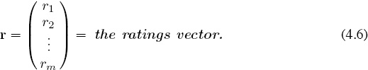
Even though the values in r are unknown to us at this point, the assumption is that they exist and can somehow be determined.
Strength
Now relate the ratings in (4.6) (which at this point exist in theory only) to the concept of “strength.” Recall that Keener’s first stipulation is that the strength of a team should be measured by how well it performs against opponents but tempered by the strength of those opponents. In other words, winning ten games against powder-puff competition shouldn’t be considered the same as winning ten games against powerful opponents.
How well team i performs against team j is precisely what your statistic aij is supposed to measure. How powerful (or powerless) team j is is what the rating value rj is supposed to gauge. Consequently, it makes sense to adopt the following definition.
It is natural to consider the overall or absolute strength of team i to be the sum of team i’s relative strengths compared to all other teams in the league. In other words, it is reasonable to define absolute strength (or simply the strength) as follows.
Absolute Strength
The absolute strength (or simply the strength) of team i is defined to be
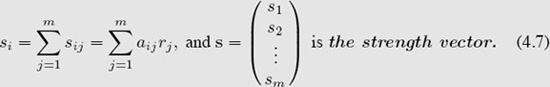
Notice that the strength vector s can be expressed as
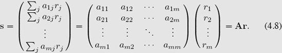
The Keystone Equation
Keener’s second stipulation concerning the relationship between strength and rating requires that the strength of each team be uniformly proportional to the team’s rating in the sense that there is a proportionality constant λ such that si = λri for each i. In terms of the rating and strength vectors r and s in (4.6) and (4.7) this says that s = λr for some constant λ. However, (4.8) shows that s = Ar, so the conclusion is that the ratings vector r is related to the statistics aij in matrix A by means of the equation
![]()
This equation is the keystone of Keener’s method!
In the language of linear algebra, equation (4.9) says that the ratings vector r must be an eigenvector, and the proportionality constant λ must be an associated eigenvalue for matrix A. Information concerning eigenvalues and eigenvectors can be found in many places on the Internet, but a recommended treatment from a printed source is [54, page 489].
At first glance, it appears that the problem of determining the ratings vector r is not only solved, but the solution from (4.9) seems remarkably easy—simply find the eigenvalues and eigenvectors for some matrix A. However, if determining r could not be narrowed down beyond solving a general eigenvalue problem Ar = λr, then we would be in trouble for a variety of reasons, some of which are listed below.
1. For a general m × m matrix A, there can be as many as m different values of λ that will emerge from the solution (4.9). This would present us with the dilemma of having to pick one value of λ over the others. The choice of λ will in turn affect the ratings vector r that is produced because once λ becomes fixed, the ratings vector r is married to it as the solution of the equation (A − λI)r = 0.
2. In spite of the fact that the matrix A of statistics contains only real numbers, it is possible that some (or even all) of the λ’s that emerge from (4.9) will be complex numbers, which in turn can force the associated eigenvectors r to contain complex numbers. Any such r is useless for the purpose of rating and ranking anything. For example, it is meaningless for one team to have rating of 6 + 5i while another team’s rating is 6 − 5i because it is impossible to compare these two numbers to decide which is larger.
3. Even in the best of circumstances in which real values of λ emerge from the solution of (4.9), they could be negative numbers. But even if a positive eigenvalue λ pops out, an associated eigenvector r can (and usually will) contain some negative entries. While having negative ratings is not as bad as having complex ratings, it is nevertheless not optimal.
4. Finally, you have to face the issue of how you are going to actually compute the eigenvalues and eigenvectors of your matrix so that you can extract r. The programming and computational complexity involved in solving Ar = λr for a general square matrix A of significant size requires most people to buy or have access to a software package that is designed for full-blown eigen computations—most such packages are so expensive that they should be shipped in gold-plated boxes.
Constraints
Keener avoids all of the above stumbling blocks by imposing three mild constraints on the amount of interaction between teams and on the resulting statistics aij in Am×m.
I. Nonnegativity. Whatever attribute you use to determine the statistics aij, and however you massage, skew, or normalize them, in the end you must ensure that each statistic aij is a nonnegative number—i.e., A = [aij] ≥ 0 is a nonnegative matrix.
II. Irreducibility. There must be enough past competition within your league to ensure that it is possible to compare any pair of teams, even if they had not played against each other. More precisely, if teams i and j are any two different teams in the league, then they must be “connected” by a a series of past contests involving other teams {k1, k2, . . . , kp} such that there is a string of games
![]()
The technical name for this constraint is to say that the competition (or the matrix A) is irreducible.
III. Primitivity. This is just a more stringent version of the irreducibility constraint in II in that we now require each pair of teams to be connected by a uniform number of games. In other words, the connection between teams i and j in (4.10) involves a chain of p games with positive statistics. For a different pair of teams, II only requires that they be connected, but they could be connected by a chain of q games with positive statistics in which p ≠ q. Primitivity requires that all teams must be connected by the same number of games—i.e., there must exist a single value p such that (4.10) holds for all i and j. The primitivity constraint is equivalent to insisting that Ap > 0 for some power p. The reason to require primitivity is because it makes the eventual computation of the ratings vector r easy to execute.
Perron–Frobenius
By imposing constraints I and II described above, the powerful Perron–Frobenius theory can be brought to bear to extract a unique ratings vector from Keener’s keystone equation Ar = λr. There is much more to the complete theory than can be presented here (and more than is needed), but its essence is given below—the complete story is given in [54, page 661].
Perron–Frobenius Theorem
If Am×m ≥ 0 is irreducible, then each of the following is true.
• Among all values of λi and associated vectors xi ≠ 0 that satisfy Axi = λixi there is a value λ and a vector x for which Ax = λx such that
![]()
• Except for positive multiples of x, there are no other nonnegative eigenvectors xi for A, regardless of the eigenvalue λi.
• There is a unique vector r (namely r = x/![]() j xj) for which
j xj) for which
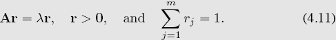
• The value λ and the vector r are respectively called the Perron value and the Perron vector. For us, the Perron value λ is the proportionality constant in (4.9), and the unique Perron vector r becomes our ratings vector.
Important Properties
Notice that by virtue of being defined by the Perron vector for A, the ratings vector r is not only uniquely determined by the statistics aij in A, but r also has the properties that each team rating is such that
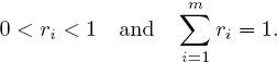
This is important because it puts everything on a level playing field in the sense that it allows for an interpretation of strength in terms of percentages—e.g., a nice pie chart can be made to graphically illustrate the strength of one team relative to the rest of the league. Having the ratings sum to one means that whenever the ratings for a particular team increases, it is necessary for one or more ratings of other teams to decrease, and thus a balance is maintained throughout a given playing season, or from year-to-year, or across different playing seasons. Furthermore, this balance allows level comparisons of ratings derived from two different attributes. For example, if we constructed one set of Keener ratings based on scores Sij and another set of Keener ratings based on wins Wij (and ties), then the two ratings and resulting rankings can be compared, reconciled, and even aggregated to produce what are sometimes called consensus (or ensemble) ratings and rankings. Techniques of rank aggregation are discussed in detail in Chapter 14.
Computing the Ratings Vector
Given that you have ensured that all statistics aij are nonnegative (i.e., A ≥ 0), then the first thing to do is to check that the irreducibility requirement described in constraint II is satisfied. Let’s assume that it is. If it isn’t, something will have to be done to fix this, and possible remedies are presented on page 39. Once you are certain that A is irreducible, then there are two options for computing r.
Brute Force. If you have access to some gold-plated numerical software that has the facility to compute eigenvalues and eigenvectors, then you can just feed your matrix A into the software and ask it to spit back at you all of the eigenvalues and all of the eigenvectors.
— Sort through the list of eigenvalues that is returned and locate the one that is real, positive, and has magnitude larger than all of the others. The Perron–Frobenius theory ensures that there must be such a value, and this is the Perron root—it is the value of λ that we are looking for.
— Next have your software return an eigenvector x that is associated with λ. This is not necessarily the ratings vector r. Depending on the software that you use, this vector x = (x1, x2, . . . , xm) could be returned to you as a vector of all negative numbers or all positive numbers (but no zeros should be present—if they are, something is wrong). Even if x > 0, its components will probably not sum to one, so you generally have to force this to happen by setting
![]()
This is the Perron vector, and consequently r is the desired ratings vector.
Power Method. If the primitivity condition in III is satisfied, then there is a relatively easy way to compute r that requires very little in the way of programming skills or computing horse power. It’s called the power method because it relies on the fact that as k increases, the powers Ak of A applied to any positive vector x0 send the product Akx0 in the direction of the Perron vector—if you are interested in why, see [54, page 533]. Consequently, scaling Akx0 by the sum of its entries and letting k → ∞ produces the Perron vector (i.e., the rating vector) r as
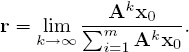
The computation of r by the power method proceeds as follows.
— Select an initial positive vector x0 with which to begin the process. The uniform vector
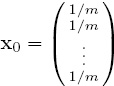
is usually a good choice for an initial vector.
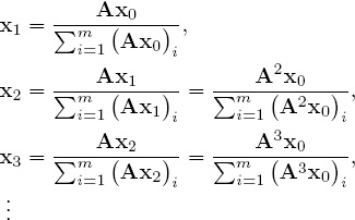
— Instead of explicitly computing the powers Ak and then applying them to x0, far less arithmetic is required by the following successive calculations. Set
![]()
It is straightforward to verify that this iteration generates the desired sequence
The primitivity condition guarantees that
xk → r as k → ∞.
(Mathematical details are in [54, page 674].) In practice, the iteration (4.12) is terminated when the entries in xk have converged to enough significant digits to draw a distinction between the teams in your league. The more teams that you wish to consider, the more significant digits you will need—see the NFL results on page 42 to get a sense of what might be required. Just don’t go for overkill. Unless you are trying to rate and rank an inordinately large number of teams, you probably don’t need convergence to 16 significant digits.
Forcing Irreducibility and Primitivity
As explained in the discussion of the constraints on page 35, irreducibility and primitivity are conditions that require sufficient interaction between the teams under consideration, and these interactions are necessary for the ratings vector r to be well defined and to be computable by the power method. This raises the natural question: “How do we actually check to see if our league (or our matrix A) has these kinds of connectivity?”
There is no short cut for checking irreducibility. It boils down to checking the definition—i.e., for each pair of teams (i, j) in your league, you need to verify that there has been a series of games
i ↔ k1 ↔ k2 ↔ . . . ↔ kp ↔ j with aik1 > 0, ak1k2 > 0, . . . , akpj > 0
that connects them. Similarly, for primitivity you must verify that there is a uniform number of games that connects each pair of teams in your league. These are tedious tasks, but a computer can do the job as long as the number of teams m is not too large.
However, the computational aspect of checking connectivity is generally not the biggest issue because for most competitions it is rare that both kinds of connectivity will be present. This is particularly true when you are building ratings (and rankings) on a continual basis (e.g., week-to-week) from the beginning of a competition and updating them throughout the playing season. It is highly unlikely that you will have sufficient connectivity to ensure irreducibility and primitivity in the early parts of the playing season, and often these connectivity conditions will not be satisfied even near or at the end of a season.
So, the more important question is: “How can we force irreducibility or primitivity into a competition so that we don’t ever have to check for it?” One particularly simple solution is to replace A by a small perturbation of itself by redefining
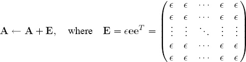
in which e is a column of all ones and ![]() > 0 is a number that is small relative to the smallest nonzero entry in the unperturbed matrix A. The effect is to introduce an artificial game between every pair of teams such that the statistics of the artificial games are small enough to not contaminate the story that the real games are trying to tell you. Notice that in the perturbed competition every team is now directly connected (with positive statistics) to every other team,1 and therefore both irreducibility and primitivity are guaranteed.
> 0 is a number that is small relative to the smallest nonzero entry in the unperturbed matrix A. The effect is to introduce an artificial game between every pair of teams such that the statistics of the artificial games are small enough to not contaminate the story that the real games are trying to tell you. Notice that in the perturbed competition every team is now directly connected (with positive statistics) to every other team,1 and therefore both irreducibility and primitivity are guaranteed.
A less stringent perturbation can be used to ensure primitivity when you know that there has been enough games played to guarantee irreducibility. If the competition (or the matrix A) is irreducible, then adding any value ![]() > 0 to any single diagonal position in A will produce primitivity. In other words, adding one artificial game between some team and itself with a negligibly small game statistic, or equivalently, redefining A as
> 0 to any single diagonal position in A will produce primitivity. In other words, adding one artificial game between some team and itself with a negligibly small game statistic, or equivalently, redefining A as
A ← A + E, where E = ![]() ei
ei![]() in which
in which ![]() = (0, 0, . . . , 1, 0, . . . , 0)
= (0, 0, . . . , 1, 0, . . . , 0)
will produce primitivity [54, page 678].
Summary
Now that all of the pieces are on the table, let’s put them together. Here is a summary of how to build rating and ranking systems from Keener’s application of the Perron–Frobenius theory.
1. Begin by choosing one particular attribute of the competition or sport under consideration that you think will be a good basis for making comparisons of each team’s strength relative to that of the other teams in the competition. Examples include the number of times team i has defeated (or tied) team j, or the number of points that team i has scored against team j.
— More than one scheme can be constructed for a given competition by taking more specific features into account—e.g., the number of rushing (or passing) yards that one football team makes against another, or the number of three-point goals or free throws that one basketball team makes against another. Even defensive attributes can be used—e.g., the number of pass interceptions that one football team makes against another, or the number of shots in basketball that team i has blocked when playing team j.
— The various ratings (and rankings) obtained by using the finer aspects of the competition can be aggregated to form consensus (or ensemble) ratings (or rankings). For example, you can construct one or more Keener schemes based on offensive attributes and others based on defensive attributes, and then aggregate the resulting ratings into one master rating and ranking list. The details describing how this is accomplished are presented in Chapter 14. Before straying off into rank aggregation, first nail down a solid system that is based on one specific attribute.
2. Whatever attribute is chosen, compile statistics from past competitions, and set
aij = the value of the statistic produced by team i when competing against team j.
It is absolutely necessary that each aij be a nonnegative number!
3. Massage the raw statistics aij in step 2 to account for anomalies. For example, if you use aij = Sij = the number of points that team i scores against team j, then as explained on page 31, you should redefine aij to be
![]()
4. If after massaging the data you feel that there is an imbalance in the sense that some aij’s are very much larger (or smaller) than they should be (perhaps due to a team artificially running up the statistics on a weak opponent), then restore a balance by constructing a skewing function such as the one in the discussion on page 31 given by
![]()
and make the replacement aij ← h(aij).
5. If not all teams have played the same number of games, then account for this by normalizing the aij’s in step 4 above by making the replacement
![]()
and organize these numbers into a nonnegative matrix A = [aij] ≥ 0.
6. Either check to see that there has been enough competition in your league to guarantee that it (or matrix A) satisfies the irreducibility and primitivity conditions defined on page 36, or else perturb A by adding some artificial games with negligible game statistics so as to force these conditions as described on page 39.
— If you are not sure (or just don’t want to check) if constraints I and II hold, then both irreducibility and primitivity can be forced by making the replacement A ← A + ![]() eeT, where e is a column of all ones and
eeT, where e is a column of all ones and ![]() > 0 is small relative to the smallest positive aij in the unperturbed A.
> 0 is small relative to the smallest positive aij in the unperturbed A.
— If irreducibility is already present—i.e., if for each pair of teams i and j there has been a series of games such that
i ↔ k1 ↔ k2 ↔ . . . ↔ kp ↔ j with aik1 > 0, ak1k2 > 0, . . . , akpj > 0
for some p (which can vary with the pair (i, j) being considered)—then the league (or matrix A) can be made primitive (i.e., made to have a uniform p that works for all pairs (i, j)) by simply adding ![]() > 0 to any single diagonal position in A. This creates an artificial game between some team and itself with a negligible statistic, and it amounts to making the replacement A ← A +
> 0 to any single diagonal position in A. This creates an artificial game between some team and itself with a negligible statistic, and it amounts to making the replacement A ← A + ![]() ei
ei![]() , where
, where ![]() > 0 and
> 0 and ![]() = (0, 0, . . . , 1, 0, . . . , 0) for some i.
= (0, 0, . . . , 1, 0, . . . , 0) for some i.
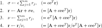
7. Compute the rating vector r by using the power method described on page 38. If you have forced irreducibility or primitivity as summarized in step 6 above, then slightly modify the power iteration (4.12) on page 38 as shown below.
— For the perturbed matrix A + ![]() eeT, execute the power method as follows.
eeT, execute the power method as follows.
• Initially set r ← (1/m)e, where e is a column of all ones.
• Repeat the following steps until the entries in r converge to a prescribed number of significant digits.
BEGIN
REPEAT
— The power method changes a bit when the perturbed matrix A + ![]() ei
ei![]() is used.
is used.
• Initially set r ← (1/m)e, where e is a column of all ones.
• Repeat the following until each entry in r converges to a prescribed number of significant digits.
BEGIN
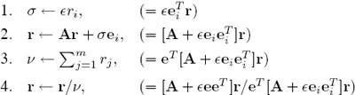
REPEAT
— These steps are simple enough that they can be performed manually in any good spreadsheet environment.
The 2009–2010 NFL Season
To illustrate the ideas in this chapter we used the scores for the regular seventeen-week 2009–2010 NFL season to build Keener ratings and rankings. The teams were ordered alphabetically as shown in the following list of team names.
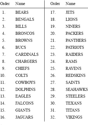
Using this ordering, we set
Sij = the cumulative number of points scored by team i against team j
during regular-season games. The matrix containing these raw scores using our ordering is shown below. For example, S12 = 10 in the following matrix indicates that the BEARS scored 10 points against the BENGALS during the regular season, and S21 = 45 means that the BENGALS scored 45 points against the BEARS.
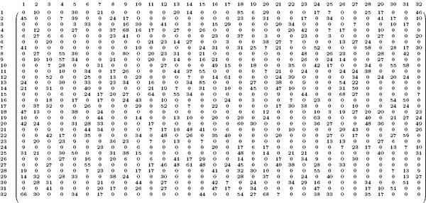
NFL 2009–2010 regular season scores
From these raw scores we used (4.2) on page 31 to construct the matrix
and then we applied Keener’s skewing function h(x) in (4.4) on page 31 to each entry in this matrix to form the nonnegative matrix
Normalization as described on page 32 is not required because all teams played the same number of games (16 of them—each team had one bye). Furthermore, A is primitive (and hence irreducible) because A2 > 0, so there is no need for perturbations. The Perron value for A is λ ≈ 15.832 and the ratings vector r (to 5 significant digits) is shown below.
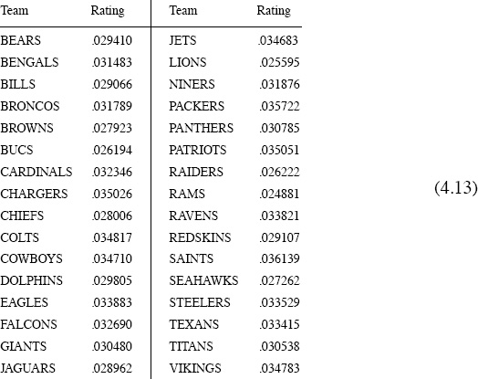
NFL 2009–2010 Keener ratings
After the ratings are sorted in descending order, the following ranking of the NFL teams for the 2009–2010 season is produced.
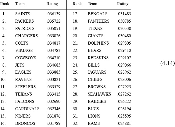
NFL 2009–2010 Keener rankings
Most who are familiar with the 2009–2010 NFL season would probably agree that this ranking (and the associated ratings) looks pretty good in that it is an accurate reflection of what happened in the post-season playoffs. The SAINTS ended up being ranked #1, and, in fact, the SAINTS won the Super Bowl! They defeated the COLTS by a score of 31 to 17. Furthermore, as shown in Figure 5.2 on page 61, the top ten teams in our rankings each ended up making the playoffs during 2009–2010, and this alone adds to the credibility of Keener’s scheme.
The COLTS were #5 in our ratings, but they probably would have rated higher if they had not rolled over and deliberately given up their last two games of the season to protect their starters from injury. It might be an interesting and revealing exercise to either delete or somehow weight the scores from the last two regular season games for some (or all) of the teams and compare the resulting ratings and rankings with those above—we have not done this, so if you follow up on your own, then please let us know the outcome.
On the other hand, after reviewing a replay of Super Bowl XLIV, it could be argued that the COLTS actually looked like a #5 team against the SAINTS, and either a healthy PATRIOTS or CHARGERS team might well have given the SAINTS a greater challenge than did the COLTS. Another interesting project would be to weight the scores so that those at the beginning of the season and perhaps some at the end do not count for as much as scores near the crucial period after midseason—and this might be done on a team-by-team basis.
Jim Keener vs. Bill James
Wayne Winston begins his delightful book [83] with a discussion of what is often called the Pythagorean theorem for baseball that was formulated by Bill James, a well-known writer, historian, and statistician who has spent much of his time analyzing baseball data. James discovered that the percentage of wins that a baseball team has in one season is closely approximated by a Pythagorean expectation formula that states
![]()
This is a widely used idea in the world of quantitative sports analysis—it has been applied to nearly every major sport on the planet. However, each different sport requires a different exponent in the formula. In other words, after picking your sport you must then adapt the formula by replacing ρ2 with ρx, where the value of x is optimized for your sport. Winston suggests using the mean absolute deviation (or MAD) for this purpose. That is, if
![]()
and
![]()
and if there are m teams in the league, then the mean absolute deviation for a given value of x is
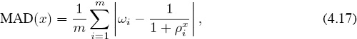
or equivalently, in terms of the vector 1-norm [54, page 274],
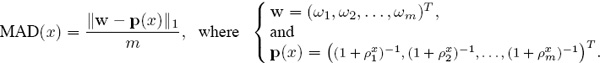
Once you choose a sport then it’s your job to find the value x* that minimizes MAD(x) for that sport. And if you are really into tweaking things, then “points” in (4.16) can be replaced by other aspects of your sport—e.g., in football it is an interesting exercise to see what happens when you use
![]()
Let’s try out James’s Pythagorean idea for the 2009–2010 NFL regular season. In other words, estimate
![]()
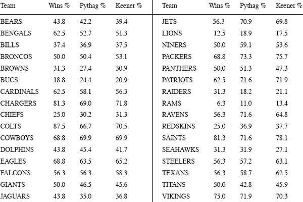
and where x is determined from the 2009–2010 NFL scoring data given on page 43. Then let’s compare these results with how well the Keener ratings in (4.13) and (4.14) estimate the winning percentages. The percentage of wins for each NFL team during the regular 2009–2010 season is shown in the following table,2 and this is our target.
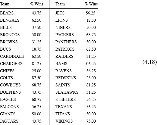
Percentage of regular-season wins for the NFL 2009–2010 season
The optimal value x* of the exponent x in (4.17) is determined by brute force. In other words, compute MAD(x) for sufficiently many different values of x and then eyeball the results to identify the optimal x*. Using the 2009–2010 NFL scoring data on page 43 we computed MAD(x) for 1500 equally spaced values of x between 1 and 4 to estimate
![]()
The graph of MAD(x) is shown in Figure 4.2. This means that the predictions produced by James’s generalized Pythagorean formula 1/(1 + ρx*) were only off by an average 6.21% per team for the 2009–2010 NFL season. Not bad for such a simple formula!
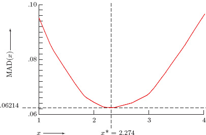
Figure 4.2 Optimal Pythagorean exponent for the NFL
Winston reports in [83] that Daryl Morey, the General Manager of the Houston Rockets, made a similar calculation for earlier NFL seasons (it’s not clear which ones), and Morey arrived at a Pythagorean exponent of 2.37. Intuition says that the optimal x* should vary with time. However, Morey’s results together with with Winston’s calculations and our value suggest that the seasonal variation of x* for the NFL may be relatively small. Moreover, Winston reports that MAD(2.37) = .061 for the 2005–2007 NFL seasons, which is pretty close to our MAD(2.27) = .062 value for the 2009–2010 season.
Now let’s see if the Keener ratings r in (4.13) on page 43 can produce equally good results. There is nothing to suggest that Keener’s ratings are Pythagorean entities that should work in any kind of nonlinear estimation formula. However, the correlation coefficient between the ratings r in (4.13) and the win percentages w in (4.18) is
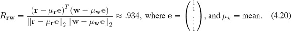
This indicates a strong linear relationship between r and the data in w [54, page 296] so rather than trying to force the ratings ri into a Pythagorean paradigm, we should be looking for optimal linear estimates of the form α + βri ≈ ωi, or equivalently αe + βr ≈ w. The Gauss–Markov theorem [54, page 448] says that “best” values of α and β are those that minimize ![]() , where A =
, where A =  , x =
, x = ![]() , and w =
, and w =  . Finding α and β boils down to solving the normal equations ATAx = AT w [54, page 226], which is two equations in two unknowns in this case. Solving the normal equations for x is a straightforward calculation that is hardwired into most decent hand-held calculators and spreadsheets. For the 2009–2010 NFL data, the solution (to five significant places) is α = −1.2983 and β = 57.545, so the least squares estimate for the percentage of regular season wins based on the Keener (Perron–Frobenius) ratings is (rounded to five places)
Est Win% for team i = α + βri = −1.2983 + 57.545 ri.
The following table shows the actual win percentage (rounded to three places) along with the Pythagorean and Keener estimates for each NFL team in the 2009–2010 regular season.
And now the punch line. The MAD for the Keener estimate is (to three significant places)
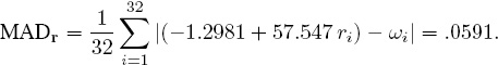
In other words, by using the Keener ratings to predict the percentage of wins in the 2009–2010 NFL season, we were only off by an average of 5.91% per team, whereas the optimized Pythagorean estimate was off by an average of 6.28% per team. MAD was used because Winston uses it in [83], but the mean squared error (or MSE) that averages the sum of squares of the errors is another common metric. For the case at hand we have
MSEPythag = .0065 and MSEKeener = .0050.
• Bottom Line. Keener (Perron–Frobenius really) wins the shootout for 2009–2010!
It is reasonable that Perron–Frobenius (aka James Keener) should be at least as good as Pythagoras (aka Bill James) because the latter does not take into account the level of difficulty (or ease) required for a team to score or to give up points whereas the former does. Is Keener’s margin of victory significant? You decide. If your interest is piqued, then conduct more experiments on your own, and let us know what you discover.
Back to the Future
Suppose that you were able to catch a ride with Marty McFly in Dr. Emmett Brown’s plutonium powered DeLorean back to the beginning of the 2009–2010 NFL season, and, just like Biff Tannen who took the 2000 edition of Grays Sports Almanac back to 1955 to make a fortune, you were able to jot Keener’s ratings (4.13) on page 43 on the palm of your hand just before you hopped in next to the flux capacitor. How many winners would you be able to correctly pick by using these ratings? Of course, the real challenge is to try to predict the future and not the past, but the exercise of looking backwards is nevertheless a valuable metric by which to gauge a rating scheme and compare it with others.
Hindsight vs. Foresight
Throughout the book we will refer to the exercise of using current ratings to predict winners of past games as hindsight prediction, whereas using current ratings to predict winners of future games is foresight prediction. Naturally, we expect hindsight accuracy to be greater than foresight accuracy, but contrary to the popular cliché, hindsight is not 20-20. No single rating value for each team can perfectly reflect all of the past wins and losses throughout the league.
Since most ratings do not account for a home-field advantage, making either hindsight or foresight predictions usually means that you must somehow incorporate a “home-field factor.” If you could take the Keener ratings (4.14) on page 44 back to the beginning of the 2009–2010 NFL season to pick winners from all 267 games during the 2009–2010 NFL season, you would have to add a home-field advantage factor of .0008 to the Keener rating for the home team to account for the fact that the average difference between the home-team score and the away-team score was about 2.4.3 By doing so you would correctly pick 196 out of the 267 games for a winning percentage of about 73.4%. This is the hindsight accuracy.
It is interesting to compare Keener’s hindsight predictions with those that might have been obtained had you taken back one of the other ratings that are generally available at the end of the season. There is no shortage of rating sites available on the Internet, but most don’t divulge the details involved in determining their ratings. If you are curious how well many of the raters performed for the 2009–2010 NFL season, see Todd Beck’s prediction tracker Web site at www.thepredictiontracker.com/nflresults.php, where many different raters are compared.
Can Keener Make You Rich?
The Keener ratings are pretty good at estimating the percentage of wins that a given team will have, but if you are a gambler, then that’s probably not your primary concern. Making money requires that a bettor has to outfox the bookies, and this usually boils down to beating their point spreads (Chapter 9 on page 113 contains a complete discussion of point spreads and optimal “spread ratings”). The “players” who are reading this have no doubt already asked the question, “How do I use the Keener ratings to predict the spread in a given matchup?” Regrettably, you will most likely lose money if you try to use Keener to estimate point spreads. For starters, the team-by-team scoring differences are poorly correlated with the corresponding differences in the Keener ratings. In fact, when 264 games from the 2009–2010 NFL season were examined, the correlation between differences in game scores and the corresponding differences in the Keener ratings was calculated from (4.20) to be only about .579. In other words, there is not much in the way of a linear relation between the two.
In fact, we would go so far as to say that it is virtually impossible for any single list of rating values to generate accurate estimates of point spreads in American football. General reasons are laid out in detail in Chapter 9 on page 113, but while we are considering Keener ratings, we might ask why they in particular should not give rise to accurate spread estimates. Understanding the answer, requires an appreciation of what is hiding underneath the mathematical sheets. In a nutshell, it is because Keener’s technique is the first cousin of a Markov chain defined by making a random walk on the thirty-two NFL teams, and as such, the ratings only convey information about expected wins over a long time horizon. Markovian methods are discussed in detail in Chapter 6 on page 67.
To understand this from an intuitive point of view, suppose that a rabid fan forever travels each week from one NFL city to another and the decision of where to go next week is determined by the entries in the matrix A = [aij] that contains your statistics. If you normalize the columns of A to make each column sum to one, then, just as suggested on page 31, aij can be thought of as the probability that team i will beat team j. But instead of using this interpretation, you can also think of aij as being
aij = Probability of traveling to city i given that the fan is currently in city j.
If aij > akj, then, relative to team j, team i is stronger than k. But in terms of our traveling fan this means that he is destined to spend a greater portion of his life in city i than city k after being in city j. Applying this logic across all cities j suggests that, in the long run, more time is spent in cities with winning teams—the higher the winning percentage, the more time spent. In other words, if we could track our fan’s movements to determine exactly what proportion of his existence is spent in each city, then we have in effect gauged the proportion of wins that each team is expected to accumulate in the long run.
The Fan–Keener Connection
The “fan ratings” rF derived from the proportion of time that a random walking fan spends in each city are qualitatively the same as the Keener ratings rK. That is, they both reflect the same thing—namely long-term winning percentages.
The intuition is as follows. The sequence x0, x1, x2, . . . generated by power method (4.12) on page 38 converges to the Keener ratings rK. Normalizing the Keener matrix at the outset to make each column sum equal one obviates the need to normalize the iterates (i.e., dividing by νk in (4.12)) at each step. The power method simplifies to become
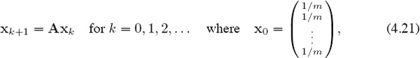
and the iterates xk estimate the path of our fan. The x0 initiates his trek by giving him an equal probability of starting in any given city. Markov chain theory [54, page 687] ensures that entry i in xk is the probability that the fan is in city i on week k. If xk → rF, then [rF]i is the expected percentage of time that the fan spends in city i over an infinite time horizon. The different normalization strategies produce small differences between rK and rF,4 but the results are qualitatively the same. Thus Keener’s ratings mirror the fan’s expected time in each city, which in turn implies that Keener reflects only long-run win percentages.
Conclusion
Keener’s ratings are in essence the result of a limiting process that reflects long-term winning percentages. They say nothing about the short-term scheme of things, and they are nearly useless for predicting point spreads. So, NO—Keener’s idea won’t make you rich by helping you beat the spread, but it was pivotal in propelling two young men into becoming two of the worlds’s most wealthy people—if you are curious, then read the following aside.
ASIDE: Leaves in the River
An allegory that appeals to us as an applied mathematicians is thinking of mathematical ideas as leaves on the tree of knowledge. A mathematician’s job is to shake this tree or somehow dislodge these leaves so that they fall into the river of time. And as they float in and out of the eddies of the ages, many will marvel at their beauty as they gracefully drift by while others will be completely oblivious to them. Some will pluck them out and weave them together with leaves and twigs that have fallen from other branches of science to create larger things that are returned to the river for the benefit and amusement of those downstream.

O. Perron

F. G. Frobenius
Between 1907 and 1912 Oskar (or Oscar) Perron (1880–1975) and Ferdinand Georg Frobenius (1849–1917) were shaking the tree to loosen leaves connected to the branch of nonnegative matrices. They had no motives other than to release some of these leaves into the river so that others could appreciate their vibrant beauty. Ranking and rating were nowhere in their consciousness. In fact, Perron and Frobenius could not have conceived of the vast array of things into which their leaves would be incorporated. But in relative terms of fame, their theory of nonnegative matrices is known only in rather specialized circles.

J. Keener
The fact that James Keener picked this shiny leaf out of the river in 1993 to develop his rating and ranking system is probably no accident. Keener is a mathematician who specializes in biological applications, and the Perron–Frobenius theory is known to those in the field because it arises naturally in the analysis of evolutionary systems and other aspects of biological dynamics. However, Keener points out in [42] that using Perron–Frobenius ideas for rating and ranking did not originate with him. Leaves from earlier times were already floating in the river put there by T. H. Wei [81] in 1952, M. G. Kendall [44] in 1955, and again by T. L. Saaty [67] in 1987. Keener’s interest in ratings and rankings seems to have been little more than a delightful diversion from his serious science. When his eye caught the colorful glint of this leaf, he lifted it out of the river to admire it for a moment but quickly let it drop back in.

Larry Page Sergey Brin
Around 1996–1998 the leaf got caught in a vortex that flowed into Google. Larry Page and Sergey Brin, Ph.D. students at Stanford University, formed a collaboration built around their common interest in the World Wide Web. Central to their goal of improving on the existing search engine technology of the time was their development of the PageRank algorithm for rating and ranking the importance of Web pages. Again, leaves were lifted from the river and put to use in a fashion similar to that of Keener. While it is not clear exactly which of the Perron–Frobenius colored leaves Brin and Page spotted in the backwaters of the river, it is apparent from PageRank patent documents and early in-house technical reports that their logic paralleled that of Keener and some before him. The mathematical aspects of PageRank and its link to Perron–Frobenius theory can be found in [49]. Brin and Page were able to exploit the rating and ranking capabilities of the Perron vector and weave it together with their Web-crawling software to parlay the result into the megacorporation that is today’s Google. With a few bright leaves plucked from the river they built a vessel of enormous magnitude that will long remain in the mainstream of the deeper waters.
These stories underscore universal truths about mathematical leaves. When you shake one from the tree into the river, you may be afforded some degree of notoriety if your leaf is noticed a short distance downstream, but you will not become immensely wealthy as a consequence. If your leaf fails to attract attention before drifting too far down the river, its colors become muted, and it ultimately becomes waterlogged and disappears beneath the surface without attracting much attention. However, it is certain that someone else will eventually shake loose similar leaves from the same branch that will attract notice in a different part of the river. And eventually these leaves will be gathered and woven into things of great value.
All of this is to make the point that the river is littered with leaves, many of similar colors and even from the same branch, but fame and fortune frequently elude those responsible for shaking them loose. The tale of Perron–Frobenius, Keener and his predecessors, and the Google guys illustrates how recognition and fortune are afforded less to those who simply introduce an idea and more to those who apply the idea to a useful end.
Historical Note: As alluded to in the preceding paragraphs, using eigenvalues and eigenvectors to develop ratings and rankings has been in practice for a long time—at least sixty years—and this area has a rich history. Some have referred to these methods as “spectral rankings,” and Sebastiano Vigna has recently written a nice historical account of the subject. Readers who are interested in additional historical details surrounding spectral rankings are directed to Vigna’s paper [79].
By The Numbers —
$8, 580, 000, 000 = Google’s Q1 2011 revenue.
— Has your interest in rating and ranking just increased a bit?
— searchenginewatch.com
1It is permissible to put zeros in the diagonal positions of E if having an artificial game between each team and itself bothers you.
2For convenience, percent numbers *% are converted by multiplying decimal values by 100.
3This is not exactly correct because while a “home team” is always designated, three games—namely on 10/25/09 (BUCS–PATRIOTS), 12/3/09 (BILLS–JETS), and 2/7/10 (COLTS–SAINTS)—were played on neutral fields, but these discrepancies are not significant enough to make a substantial difference.
4The intuition is valid for NFL data because the variation in the column sums of Keener’s A is small, so the alternate normalization strategy amounts to only a small perturbation. The difference between rK and rM can be larger when the variation in the column sums in A is larger.