
Chapter Seven
The Offense–Defense Rating Method
A natural approach in the science of ratings is to first rate individual attributes of each team or participant, and then combine these to generate a single number that reflects overall strength. In particular, success in most contests requires a strong offense as well as a strong defense, so it makes sense to try to rate each separately before drawing conclusions about who is #1.
But this is easier said than done, especially with regard to rating offensive strength and defensive strength. The problem is, as everyone knows, playing against a team with an impotent defense can make even the most anemic offense to appear stronger than it really is. And similarly, the apparent defensive prowess of a team is a direct consequence on how strong (or weak) the opposition’s offense is. In other words, there is a circular relationship between perceived offensive strength and defensive strength, so each must take the other into account when trying to separately rate offensive power and defensive power. How this is accomplished is the point of this chapter.
OD Objective
The objective is to assign each team (or participant) both an offensive rating (denoted by oi > 0 for team i) and a defensive rating (denoted by di > 0 for team i) that are derived from statistics accumulated from past play. Given any particular sport or contest, there are generally many statistics that might be considered, but scores are the most basic statistics, and actually they do a pretty good job. Moreover, once you understand how our OD method uses scores to produce offensive and defensive ratings, you will then easily see how to use statistics other than scores to build your own systems. For these reasons, we will describe our OD rating technique in terms of scores.
OD Premise
Suppose that m teams are to be rated, and use scoring as the primary measure of performance. Team j is considered to be a good offensive team and deserves a high offensive rating when it scores many points against its opponents, particularly opponents with high defensive ratings. Similarly, team i is a good defensive team and deserves a high defensive rating when it holds its opponents, particularly strong offensive teams, to low scores. Consequently, offensive and defensive ratings are intertwined in the sense that each offensive rating is some function f of all defensive ratings, and each defensive rating is some function g of all offensive ratings.
So, the issue now boils down to determining how the functions f and g should be defined. Since scoring is going to be the primary measure of performance, organize past scores into a score matrix A = [aij] in which aij is the score that team j generated against team i (average the results if the teams met more than once, and set aij = 0 if the two teams did not play each other). Notice that aij has a dual interpretation in the sense that
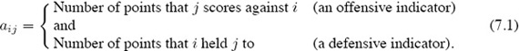
In other words, depending on how it is viewed, aij simultaneously reflects relative offensive and defensive capability. This dual interpretation is used to formulate the following definitions of f and g for each team.
The OD Ratings
For a given set of defensive ratings {d1, d2, . . . , dm}, define the offensive rating for team j to be
![]()
Similarly, for a given set of offensive ratings {o1, o2, . . . , om}, define the defensive rating for team i to be
![]()
Reflect on these definitions for a moment to convince yourself that they make sense by reasoning as follows. To understand the offensive rating, suppose that team * has a weak defense. Consequently, d* is relatively large. If team j runs up a big score against team *, then a*j is large. But this large score is moderated by the large d* in the term a*j/d* that appears in the definition of oj. In other words, scoring a lot of points against a weak defense will not contribute much to the total offensive rating. But if team * has a strong defense so that d* is relatively small, then a large score against * will not be mitigated by a small d*, and a*j/d* will significantly increase the offensive rating of team j.
The logic behind the defensive rating is similar. Holding a strong offense to a low score drives the term ai*/o* downward in the defensive rating for team i, but allowing a weak offense to run up the score produces a larger value for ai*/o*, which contributes to a larger defensive rating for team i.
But Which Comes First?
Since the OD ratings are circularly defined, it is impossible to directly determine one set without knowing the other. This means that computing the OD ratings can only be accomplished by successive refinement in which one set of ratings is arbitrarily initialized and then successive substitutions are alternately performed to update (7.2) and (7.3) until convergence is realized.
Alternating Refinement Process
Initialize the defensive ratings with positive values stored in a column vector d0. These initial ratings can be assigned arbitrarily—we will generally set
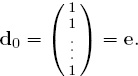
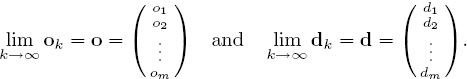
Use the values in d0 to compute a first approximation to the offensive ratings from (7.2), and store the results in a column vector o1. Now use these values to compute refinements of the defensive ratings from (7.3), and store the results in a column vector d1. Repeating this alternating substitution process generates two sequences of vectors
![]()
If these sequences converge, then the respective offensive and defensive ratings are the components in the vectors
To better analyze this alternating refinement process it is convenient to describe the vectors in this sequence by using matrix algebra along with a bit of nonstandard notation. Given a column vector with positive entries
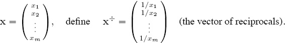
If A = [aij] is the score matrix defined in (7.1), then the OD ratings in (7.2) and (7.3) are written as the two matrix equations
![]()
and
![]()
Consequently, with d0 = e, the vectors in the OD sequences (7.4) are defined by the alternating refinement process
![]()
and
![]()
The Divorce
The interdependence between the ok’s and dk’s is easily broken so that the computations need not bounce back and forth between offensive and defensive ratings. This is accomplished with a simple substitution of (7.8) into (7.7) to produce the following two independent iterations.
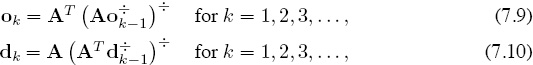
where o0 = e = d0.
However, there is no need to use both of these iterations because if we can produce ratings from one of them, the other ratings are obtained from (7.5) or (7.6). For example, if the offensive iteration (7.9) converges to o, then plugging it into (7.6) produces d. Similarly, if we only iterate with (7.10), and it converges to d, then o is produced by (7.5).
Combining the OD Ratings
Once a set of offensive and defensive ratings for each team or participant has been determined, the next problem is to decide how the two sets should be combined to produce a single rating for each team? There are many methods for combining or aggregating rating lists—in fact, Chapters 14 and 15 are devoted to this issue. But for the OD ratings, the simplest (and perhaps the most sensible) thing to do is to define an aggregate or overall rating to be
![]()
In vector notation, the overall rating vector can be expressed as r = o/d, where / denotes component-wise division. Remember that strong offenses are characterized by big oi’s while strong defenses are characterized by small di’s, so dividing the offensive rating by the corresponding defensive rating makes sense because it allows us to retain the “large value is better” interpretation of the overall ratings in r.
Our Recurring Example
Put the scores in Table 1.1 from our recurring five-team example on page 5 into a scoring matrix
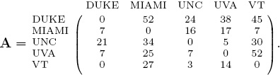
Starting with d0 = e and implementing the alternating iterative scheme in (7.8)–(7.7) requires k = 9 iterations to produce convergence of both of the OD vectors to four significant digits. The results are shown in the following table.
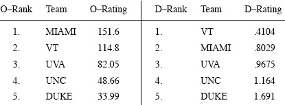
OD ratings for the 5-team example
It is clear from these OD ratings and rankings that UVA, UNC, and DUKE should be respectively ranked third, fourth, and fifth overall. However, the OD rankings for VT and MIAMI are flip flopped, so their positions in the overall rankings are not evident. But using the OD ratio in (7.11) resolves the issue. The overall ratings are shown below.
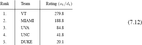
Overall ratings for the 5-team example
Scoring vs. Yardage
As mentioned in the introduction to this chapter, almost any statistic derived from a competition could be used in place of scores. For football, it is interesting to see what happens when scores are replaced by yards gained (or given up) in our OD method. As part of his M.S. thesis [41] at the College of Charleston, Luke Ingram used the 2005 ACC Football scoring and yardage data to investigate this issue. The scoring data in our small five-team recurring example is a subset of Luke’s experiments. Using a similar subset of Luke’s yardage data for the same five teams yields the yardage matrix
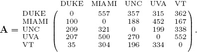
in which
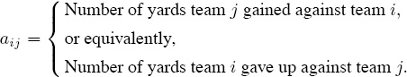
Starting with d0 = e and implementing the alternating iterative scheme in (7.8)–(7.7) requires k = 6 iterations to produce convergence of both of the OD vectors to four significant digits when the yardage data is used. The results are shown below.
OD ratings for the 5-team example when yardage is used
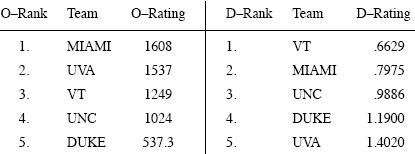
This time things are not as clearly defined as when scores are used. The overall ratings obtained from the yardage data is as follows.
Overall ratings for the 5-team example when yardage is used
The results in (7.12) are similar to those in (7.13) except that MIAMI and VT have traded places. Experiments tend to suggest that scoring data provides slightly better overall rankings (based on the final standings) for NCAA football than does yardage data. Perhaps this is because the winner is the team with the most points, not necessarily the team with the most total yardage. However, OD ratings based on yardage can be a good indicator of overall strength at particular times in the midst of a season. Of course, results will differ in other sports settings or competitions.
The 2009–2010 NFL OD Ratings
Since we have used the 2009–2010 NFL data in some examples in other places in this book, you might be wondering what the OD ratings look like for the 2009–2010 NFL season. The offensive and defensive ratings were computed using the scoring data for all games (including playoff games), and scores were averaged when two teams played against each other more than once. The results are shown in the following tables.

Offensive ratings for the 2009–2010 NFL season when scoring is used

Defensive ratings for the 2009–2010 NFL season when scoring is used
If the ratio ri = oi/di is used to aggregate the offensive and defensive ratings to produce a single overall rating for each team, then the results for the 2009–2010 NFL season are as follows.
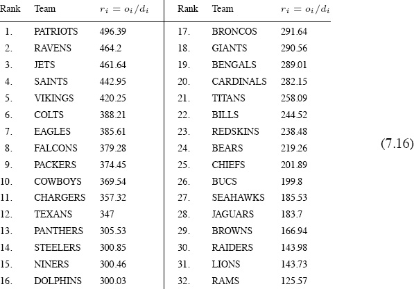
Overall ratings for the 2009–2010 NFL season determined by the ratio O/D
However, using this simple ratio is not the only (nor necessarily the best) way to aggregate the OD ratings. For example, it puts as much importance on offense as defense. If you want to experiment with some more complicated strategies, then you might try to build some sort of regression model such as
α(oh − ow) + β(dh − da) = sh − sa,
where oh, dh, oa, da are the respective OD ratings for the home and away teams, and sh and sa are the respective scores. Warning! Once you start tinkering with ideas like this, you will find that they become infectious. In fact, they are quicksand, and your personal relationships along with your performance at your day job may suffer.
The NFL is not be the best example to illustrate the benefits of our OD method because the NFL is extremely well balanced—much more so than most other sports. The league goes to great lengths to insure this. Consequently, the differentiation between weak and strong offenses (and defenses) is not nearly as pronounced as it is in NCAA competition or in other sports. This means that you won’t be too far off the mark by just using raw score totals (without regard to the level of the competition) to gauge offensive and defensive prowess in the NFL, but in other sports or competitions this may not be the case. For example, when the same scoring matrix A that produces the NFL OD ratings shown above is used to compute
![]()
and
![]()
the following results are produced.
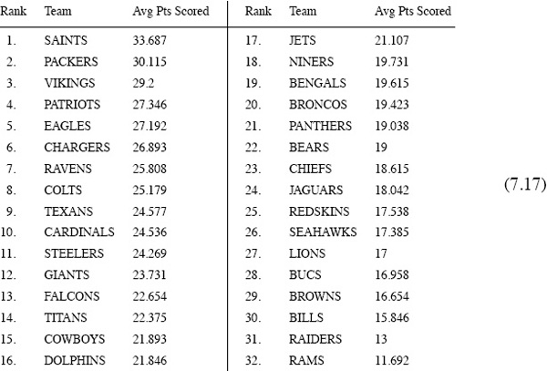
Average points scored per game during the 2009–2010 NFL season
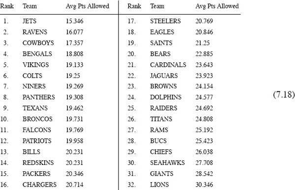
Average points allowed per game during the 2009–2010 NFL season
If you take a moment to compare the offensive ratings in (7.14) with average points scored in (7.17), you see that while they do not provide exactly the same rankings, they are nevertheless more or less in line with each other—as they should be. Something would be amiss if this were not the case because the same data produced both sets of rankings. The difference is that offensive ratings in (7.14) take the level of competition into account whereas the raw scores in (7.17) do not. Similarly, the defensive ratings (7.15) are more or less in line with the average points allowed shown in (7.18)—all is right in the world.
Mathematical Analysis of the OD Method
The algorithm for computing the OD ratings is really simple—you just alternate the two multiplications (7.7) and (7.8) as described on page 81. Among all of the rating schemes discussed in this book, our OD method is one of the easiest to implement—an ordinary spread sheet can comfortably do this for you, or, if there are not too many competitors, a hand calculator or even pencil-and-paper will do the job. However, the simplicity of implementation belies some of the deeper mathematical issues surrounding the theory of the OD algorithm.
The main theoretical problem concerns the existence of the OD ratings. Since the vectors o and d that contain the OD ratings are defined to be the limits
![]()
where
![]()
there is a real possibility that o and d may not exist—indeed, there are many cases in which these sequences fail to converge.
A theorem is needed to tell us when convergence is guaranteed and when convergence is impossible. Before developing such a theorem, some terminology, notation, and background information are required. Things hinge on the realization that the OD method is closely related to a successive scaling or balancing procedure on the data matrix Am×m. To understand this, suppose that the columns of A are first scaled (or balanced) to make all column sums equal to one, and then the resulting matrix is row-scaled to make all row sums equal to one. This can be described as multiplication with diagonal scaling matrices C1 and R1 such that AC1 has all column sums equal to one followed by R1(AC1) to force all row sums equal to one. In other words, if
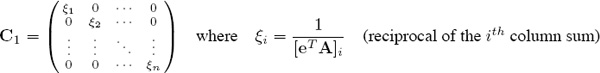
and
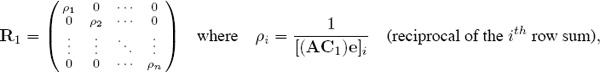
then
R1AC1e = e (i.e., all row sums are one).
Unfortunately, scaling the rows of AC1 destroys the column balance achieved in the previous step when we multiplied A by C1—i.e., the column sums of R1AC1 are generally not equal to one. However, the column sums in R1AC1 are often closer to being equal to one than those of A. Consequently, the same kind of alternate scaling is performed again, and again, and again, until the data is perfectly balanced in the sense that the row sums as well as the column sums are all equal to one (or at least close enough to one within some prescribed tolerance). Successive column scaling followed by row scaling generates a sequence of diagonal scaling matrices Ck and Rk such that
Sk = Rk · · · R2R1AC1C2 · · · Ck ≥ 0 where Ske = e (all row sums are one).
A square matrix S having nonnegative entries and row sums equal to one is called a stochastic matrix. When the row sums as well as the column sums in S are all equal to one, S is said to be a doubly stochastic matrix.
Thus the matrix Sk = Rk · · · R2R1AC1C2 · · · Ck resulting from successive column and row scalings is a stochastic matrix for every k = 1, 2, 3, . . . . The hope is that S = limk→∞ Sk exists and S is doubly stochastic. Alas, this does not always happen, but all is not lost because there is a theorem that tells us exactly when it will happen. Understanding the theorem requires knowledge of the “diagonals” in a square matrix.
Diagonals
The main diagonal of a square matrix A is the set of entries {a11, a22, . . . amm}, and this is familiar to most people. However, there are other “diagonals” in A that receive less notoriety. In general, if σ = (σ1, σ2, . . . , σm) is a permutation of the integers (1, 2, . . . , m), then the diagonal of A associated with σ is defined to be the set
{a1σ1, a2σ2, . . . amσm}.
For example, in ![]() the main diagonal {1, 5, 9} corresponds to the natural order (1, 2, 3), while this and all other diagonals are derived from the six permutations as shown below.
the main diagonal {1, 5, 9} corresponds to the natural order (1, 2, 3), while this and all other diagonals are derived from the six permutations as shown below.

Sinkhorn–Knopp
In 1967 Richard Sinkhorn and Paul Knopp [70] proved a theorem that perfectly applies to the OD theory. Their theorem is as follows.
Sinkhorn–Knopp Theorem
Let Am×m be a nonnegative matrix.
• The iterative process of alternately scaling the columns and rows of A will converge to a doubly stochastic limit S if and only if there is at least one diagonal in A that is strictly positive, in which case A is said to have support.
This statement guarantees the scaling process will converge to a doubly stochastic matrix, but it does not ensure that the products Ck = C1C2 · · · Ck and Rk = Rk · · · R2R1 will converge—e.g., successively scaling ![]() converges to I (the identity), but Ck and Rk do not converge.
converges to I (the identity), but Ck and Rk do not converge.
• The limits of the diagonal matrices
![]()
exist and RAC = S is doubly stochastic if and only if every positive entry in A lies on a positive diagonal, in which case A is said to have total support.
OD Matrices
As discussed on page 83, statistics other than game scores (such as yardage in football) can be used to compute OD ratings. Throughout the rest of the OD development, it will be understood that Am×m is a matrix of nonnegative statistics (scores, yardage, etc.), and such a matrix will be called an OD matrix. The major observation is that applying the Sinkhorn–Knopp process to an OD matrix produces OD ratings by reciprocation. This is developed in the following theorem.
The OD Ratings and Sinkhorn–Knopp
In subsequent discussions it is convenient to identify column vectors x with associated diagonal matrices by means of the mapping
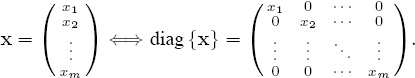
Notice that diag {x} e = x = eT diag {x}. Furthermore, for vectors v with nonzero components and for diagonal matrices D with nonzero diagonal elements, it is straightforward to verify that
![]()
We are now in a position to prove the primary OD theorem that tells us when the OD rating vectors exist and when they do not.
The OD Theorem
For an OD matrix Am×m, the OD sequences
![]()
respectively converge to OD rating vectors o and d if and only if every positive entry in A lies on a positive diagonal—i.e., if and only if A has total support.
Proof. As in earlier discussions, let Ck and Rk denote the respective products
Ck = C1C2 · · · Ck and Rk = Rk · · · R2R1
of the diagonal scaling matrices generated by the Sinkhorn–Knopp process. The key is to establish a connection between these products and the OD sequences in (7.21). To do this, recall that the diagonal scaling matrices in the Sinkhorn–Knopp process are generated as follows.
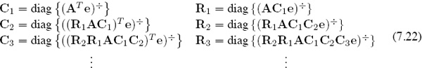
Observe that the products Ck and Rk can be expressed as
![]()
![]()
This can be verified by writing out the first few iterates. For example, c1 = (AT e)÷, so it is clear from (7.22) that C1 = diag {c1}, and C1e = c1, and thus
R1 = diag (AC1e)÷ = diag (Ac1)÷ = diag {r1}.
Use this along with (7.20) to write

so that C2 = C1C2 = diag {c2}. Similarly, this together with (7.20) yields
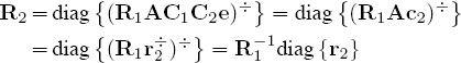
so that R2 = R2R1 = diag {r2}. Proceeding inductively establishes (7.23). Now observe that the sequences in (7.24) are simply the reciprocals of the OD sequences in (7.21). In other words,
![]()
Again, this is easily seen by writing out the first few terms as shown below and proceeding inductively.

The Sinkhorn–Knopp Theorem on page 89 says that the limits
![]()
exist if and only if A has total support. Consequently, (7.23) means that the limits
![]()
exist if and only if A has total support, and thus (7.25) ensures that the limits
![]()
exist if and only if A has total support. ![]()
Cheating a Bit
Not all OD matrices will have the total support property—i.e., not every positive entry will lie on a positive diagonal. Without total support, the OD rating vectors cannot exist because the defining sequences will not converge, so it is only natural to try to cheat a bit in order to force convergence. One rather obvious way of cheating a little is to simply add a small number ![]() > 0 to each entry in A. That is, make the replacement
> 0 to each entry in A. That is, make the replacement
A ← A + ![]() eeT > 0.
eeT > 0.
This forces all entries to be positive, so total support is automatic, and thus convergence of the OD sequences is guaranteed. If it bothers you to add something to the main diagonal of A because it suggests that a team has beaten itself, you can instead make the replacement
A ← A + ![]() (eeT − I),
(eeT − I),
which will also guarantee total support.
If ![]() is small relative to the nonzero entries in the original OD matrix, then the spirit of the original data will not be overly compromised, and the OD ratings produced by the slightly modified matrix will still do a good job of reflecting relative offensive and defensive strength. However, there is no free lunch in the world, and there is a price to be paid for this bit of deception.
is small relative to the nonzero entries in the original OD matrix, then the spirit of the original data will not be overly compromised, and the OD ratings produced by the slightly modified matrix will still do a good job of reflecting relative offensive and defensive strength. However, there is no free lunch in the world, and there is a price to be paid for this bit of deception.
While relative offensive and defensive strengths are not overly distorted by a small perturbation, the rate of convergence can be quite slow. It should be intuitive that as ![]() becomes smaller, the number of iterations needed to produce viable results grows larger. In other words, you need to walk a tightrope by balancing the desired quality of your OD ratings against the time you are willing to spend to generate them. However, keep in mind that you may not need many significant digits of accuracy to produce useable ratings.
becomes smaller, the number of iterations needed to produce viable results grows larger. In other words, you need to walk a tightrope by balancing the desired quality of your OD ratings against the time you are willing to spend to generate them. However, keep in mind that you may not need many significant digits of accuracy to produce useable ratings.
As demonstrated in (7.25), the OD sequences are nothing more (or less) than the reciprocals of the Sinkhorn–Knopp sequences in (7.24), so the rate of convergence of the OD sequences is the same as convergence rates of the Sinkhorn–Knopp procedure. While estimates of convergence rates of the Sinkhorn–Knopp have been established, they are less than straightforward. Some require you to know the end result of the process so that you cannot compute an a priori estimate while others are “order estimates” where the order constants are not known or not computable. A detailed discussion of convergence characteristics would take us too far astray and would add little to the application of the OD method. Technical convergence discussions are in [30, 46, 72, 73]. Additional information and applications involving the OD method can be found in Govan’s work [34, 35].
ASIDE: HITS
Our OD method is a nonlinear cousin of Jon Kleinberg’s algorithm called HITS (Hypertext Induced Topic Search) [45] that was designed for ranking linked documents. HITS became a pivotal technique for ranking the most popular type of linked documents, webpages. The HITS idea was incorporated into the search engine Ask.com. HITS, like many search engine models, views the Web as a gigantic directed graph. As observed in several places in this book, the interaction between competitive contests can also be viewed as a large graph. Consequently, some webpage ranking algorithms can be adapted to create rankings (and vice versa). A detailed discussion of HITS for ranking webpages is given in [45] and [49], but here is the basic idea in a nutshell. Each webpage, which in Figure 7.1 is represented by a node, is given both a “hub rating” and an “authority rating.” A hub rating is meant to reflect the quality and quantity of a Web page’s outlinks, while the authority rating measures the quality and quantity of its inlinks. The intuition is that hub pages act as central points in the Web that provide users with many good links to follow—e.g., YAHOO! has many good hub pages. Authorities are pages that are generally informative and many good sites point to them—e.g., WIKIPEDIA has many good authority pages. A page’s hub rating depends on the authority ratings of the pages it links to. In turn, a page’s authority rating depends on the hub rating of those pages linking to it. Kleinberg called this a “mutually reinforcing” rating system because one rating is dependent on the other—do you notice the similarity with OD? To compute hub and authority ratings, start with a square adjacency matrix L, where

J. Kleinberg
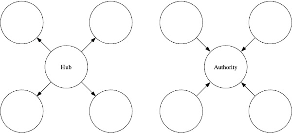
Figure 7.1 Hub page and an authority page
![]()
Choose an arbitrary initial authority rating vector (the uniform vector a0 = e is often used) and successively refine hub and authority ratings by setting
![]()
These equations make the dependency between authority and hub ratings clear. This interdependence is broken by exactly the same “divorce” strategy that was described on page 81. That is, substitute the expression for hk into the equation defining ak+1 to get
ak+1 = LT Lak and hk+1 = LLT hk.
Provided that they converge, the limits of these two sequences provide the desired hub and authority ratings. Readers interested in more details concerning implementation, code, and extensions of HITS should consult Chapter 11 in [49].
ASIDE: The Birth Of OD
During our work on the “Google book” [49] concerning the PageRank algorithm, we often mused over the possibilities of applying Web-page rating and ranking ideas to sports. After all, search-engine ranking methods are themselves just adaptations of basic principles from other disciplines (e.g., bibliometrics), so, instead of ranking Web pages, why couldn’t the same ideas be applied to sports applications? Of course, they can. The Markovian methods discussed in Chapter 6 on page 67 are straightforward adaptions of the PageRank idea. But what about other Web-page ranking techniques? One afternoon in 2005 we were kicking these thoughts around, and Kleinberg’s HITS came up. As described above, HITS is an elegantly simple idea, and although it doesn’t scale up well, it is nevertheless effective for small collections—perhaps even superior to PageRank. It seemed natural to reinterpret Kleinberg’s “hubs-authorities” concept as an “offense-defense” scheme. However it soon became apparent that a direct translation from hubs-and-authorities to offense-and-defense was not workable. But the underlying idea was too pretty to give up on, so the wheels continued to spin. It did not take long to realize that while hubs and authorities are linearly related as described in (7.26), the relationship between offense and defense is inherently nonlinear, and some sort of reciprocal relationship had to be formulated. After that, the logic flowed smoothly, and thus the OD method was born.

A. Govan
Shortly thereafter Anjela Govan arrived at NC State as a graduate student to study Markovian methods in data analytics, but in the course of casual conversation she became intrigued by rating and ranking. In spite of advice concerning the dubiousness of pursuing a thesis motivated by football, she followed her heart and went on to develop the connections between the OD method and the Sinkhorn–Knopp theory, which, as described in the discussion beginning on on page 87, provides the theoretical foundation for analyzing the mathematical properties of the OD method. In addition, she was instrumental in developing and analyzing several of the Markovian methods discussed in this book as well as several that were not elaborated here. And her adept programming ability produced substantial and innovative web-scraping software to automatically harvest data from diverse web sites. This alone was a significant achievement because the countless number of numerical experiments that were subsequently conducted would have been more difficult without the use of her tools.
ASIDE: Individual Awards in Sports
At the end of the season, many sports crown players with individual awards. For instance, college football selects a winner for its prestigious Heisman trophy. Collegiate and professional basketball select all-offensive and all-defensive teams. Such selections are generally made by compiling and combining votes from coaches, sports writers, and sometimes even fans. These selections could easily be supplemented by the addition of scientific ranking methods such as those found in this book. However, it is not a trivial issue to select the most appropriate ranking method for a particular award. Some careful thought and clever mathematical modeling is required to achieve the appropriate aim of the award. For instance, the Markov model in Chapter 6 is a good choice for selecting an all-defensive team, whereas the OD method of this chapter might be most appropriate for the Player of the Year award, since OD incorporates both offensive and defensive ability. There are many parameters for tweaking and tailoring the models, making this an exciting avenue of future work.
ASIDE: More Movie Rankings: OD Meets Netflix
The aside “Movie Rankings: Colley and Massey meet Netflix” on page 25 introduced the Netflix Prize. Netflix sponsored a $1 million prize to improve its current recommendation system. The prize was claimed in September 2009 by the “BellKor” team of researchers. The earlier Netflix aside described how the Colley and Massey methods could be used to rank movies. In this aside, we describe how the OD method can be modified to do the same. In fact, since the matrix in this case is rectangular and OD gives dual rating vectors, we will get both a movie rating vector m and a user rating vector u. Below we have chosen to display only the top-24 elements of the movie rating vector m. The final user rating vector u and its corresponding ranking of users are of little interest to us, of course, u is of great interest to companies such as Netflix that build marketing strategies around such user information. The Netflix OD method begins with the thesis that movie i is good and deserves a high rating mi if it gets high ratings from good (i.e., discriminating) users. Similarly, user j is good and serves a high rating uj when his or her ratings match the “true” ratings of the movies. One mathematical translation of these linguistic statements produces the iterative procedure below, which is written in MATLAB style. There are several methods for quantifying the phrase “discriminating user” (see, for instance, some of the approaches of the Netflix prize winners) but one elementary approach tries to measure how far a user’s ratings are from the true ratings.
    u = e;
    for i = 1 : maxiter
         m = A u;
         m = 5 (m−min(m)) / (max(m) −min(m)) ;
         u = 1 / ((R −(R>0) . * (em′)).^2)e
    end
Applying this algorithm to a subset of Netflix data, specifically the ratings of “power users,”1 i.e., those users who have rated 1000 or more movies, results in the following top-24 list of movies. This list is considerably different than the lists on page 28 produced by the Colley and Massey methods.
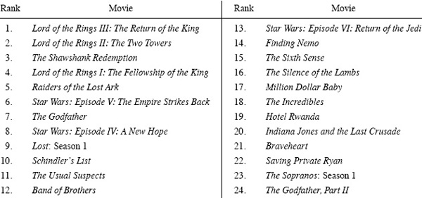
Top-24 movies ranked by Netflix OD method
$3, 142, 000, 000 = total amount wagered on sports in Nevada in 2010.
— The Line Makers
1It was surprising for us to learn just how many power users there are in the Netflix dataset. There are over 13,000 users who have rated more than a thousand movies.