Chapter Eleven

Handling Ties

Companies such as Amazon, Netflix, and eBay solicit and collect data on user behavior, which results in enormous databases with records of user ratings of products and services. One common goal of analyzing this data is to create rankings of items, which may then be used as part of a recommendation system. Typically, the first step in creating such a ranking is to transform the user ratings into pair-wise comparisons. There are several methods for doing this. See, for instance, [33] and the material in Chapter 10. Every transformation begins by creating head-to-head contests between pairs of items. For example, in a database of user ratings about movies, the (i, j)-element of a possible pair-wise matrix could contain the number of times movie i beat movie j in their contests, where a contest occurs each time a user has rated both movies. As a result, it is clear that ties are prevalent in many database applications.

This chapter discusses ranking in the presence of ties in the input data, and many of the results are compilations of those in [20]. Ties can also exist in the output (the final rankings)—more on this topic appears in Chapter 15. The issue of how to handle ties in the input data has received little attention despite the fact that this decision can have a significant impact on ranking results. Many ranking methods handle ties by simply ignoring them. Here are three compelling reasons for a more careful consideration of ties.

• Depending on the application, ties can comprise a sizeable portion of the data. For most NHL seasons, 9–13% of games end in ties. Ties are much more prevalent in database applications. For example, when ranking movies rated by users, it is typical to find that up to 50% of the “game” data in this context are ties. In this scenario, a game occurs when two movies have both been rated by the same user. The movie receiving the higher rating wins that “game.”

• Some methods, such as the Massey method, incorporate ties while others, such as the Colley method, ignore them. Thus, when comparing rankings produced by various methods, it is important to make the comparison fair by treating ties uniformly across all methods. We advocate accounting for, rather than ignoring, ties. When ties are accounted for, a low-ranked team that ties a high-ranked team is rewarded for its effort while the high-ranked team is penalized. This reaction to the tie has more intuitive appeal than treating it as a non-event.

• There are some sports where ties are rare or impossible due to overtime or shootout rules. In such sports, it sometimes happens that two teams were very evenly matched for the large duration of the game, yet one emerged the victor due to a last minute heroic. On page 142, we induce ties for these near-tied events and other near-tied events such as those with very small point differentials. We show that these induced ties can improve the predictive power of the ranking results. In applications such as the BCS rankings of college football teams, small changes in the ranking results can have huge impacts on universities, given the revenue associated with bowl invitations.

Input Ties vs. Output Ties

In general, ties have received very little attention in the ranking literature. Here we distinguish between two types of ties. Input ties are ties in the input data (i.e., games that end in a tied score) and output ties that are ties in the output data (i.e., when a ranking method outputs a ranking that contains ties). Some work has been done regarding output ties, particularly in the context of rank aggregation [3, 4, 23, 27, 50]. Rank aggregation is related to, yet different from, ranking. Rank aggregation, which is also known as consensus ranking, creates one ranking that is an aggregate of several other rankings. See Chapters 14 and 15 for more on rank aggregation. In contrast, in this chapter, we are interested in input ties and their effect on ranking, not rank-aggregation, methods.

Incorporating Ties

For a ranking application in which the data contains ties, one must be very careful when comparing rankings produced by different methods. Some methods, such as the Massey and OD methods, very naturally account for ties, while others, such as the Colley and some Markov variants, ignore them. All methods either already incorporate or can be modified to use information from ties. Consequently, in order to make fair comparisons across methods, for each method, one must derive two models: one when ties are used and another when ties are omitted.

The Colley Method

Recall from Chapter 3 that the Colley method can be succinctly summarized with one linear system, Cr = b, where r_n×1 is the unknown Colley rating vector, b_n×1 is the right-hand side vector defined as b_i = 1 + (w_i − l_i) and C_n×n is the Colley coefficient matrix defined as

The scalar n_ij is the number of times teams i and j played each other, t_i is the total number of games played by team i, w_i is the number of wins for team i, and l_i is the number of losses for team i.

Since the Colley method only accounts for wins and losses, ties are, in effect, non-events that are ignored. Thus, we now refer to the above model as the Colley-no-ties method. In order to incorporate ties, we must modify the above model, creating the Colleyties method.

Incorporating ties into the Colley method requires some thought as to the meaning of a tied outcome. One interpretation of a tie argues that, if the two teams were to meet again, there would be an equal chance that either team would win. Or complementarily, we could say that there is an equal chance that either team would lose. Thus, to include ties we count a tie between teams i and j as two games, dividing the usual weight of 1 equally between the two artificial games. In one artificial game, team i beats team j with a weight of 1/2 while in the other team j beats team i. This interpretation of a tie leaves the b vector unaltered and modifies the C matrix in an obvious way (i.e., for a tie between teams i and j, c_ij and c_ji decrement by 1 and c_ii and c_jj increment by 1). One nice consequence of this interpretation of ties is that the Colley conservation property, which states that the sum of all Colley ratings is n/2, is maintained.

The Massey Method

Recall from Chapter 2 that the Massey method can be succinctly summarized with the linear system

Mr = p,

where the Massey coefficient matrix M is related to the Colley matrix C by the formula M = C − 2I so that

The Massey right-hand side vector p is a vector of cumulative point differentials. That is, p_i is the total number of points team i scored on all opponents minus the total number of points opponents scored against team i. Since rank(M) = n − 1, an adjustment is made to ensure nonsingularity. Any row of M is replaced with a row of all 1s and the corresponding entry in p is set to 0. This new constraint forces the ratings to sum to 0. Following Massey’s advice, we apply this nonsingularity adjustment to the last row, creating an adjusted linear system which we denote .

The above Massey method naturally incorporates ties. For a tied event between teams i and j, the m_ij and m_ji entries increment by one, yet the information in the point differential vector p remains unchanged. Thus, we refer to the above method as the Massey-ties method.

In order to properly analyze the methods there needs to be a comparable Massey-noties method that does not incorporate ties in creating the rating. To accomplish this with minimal change, alter the Massey method to ignore any game that ends in a tie. That is, we do not update the M matrix or p vector when a tie occurs between teams i and j. This behaves similar to the Colley-no-ties method in that these ties are considered non-events.

The Markov Method

The key to the Markov method of Chapter 6 is voting. A weaker team casts votes for each stronger team it faces, and because there are several methods for vote casting, the Markov method has several variants. In this chapter, we consider the following three.

1. A losing team casts one vote for each team it is beaten by.

2. A losing team casts a number of votes equal to the number of points it was beaten by.

3. For each game, both winning and losing teams cast a number of votes equal to the number of points given up.

 

Regardless of the vote casting method, the result is a team-team matrix that is row-normalized in order to enforce stochasticity, which creates the transition matrix for a Markov chain. The stationary vector of this chain is the Markov rating vector. As discussed in Chapter 6, the elements of the stationary vector correspond to the proportion of time one would visit a particular team if one took a random walk on the graph defined by the voting matrix. The higher the rating (i.e., the higher the value in the stationary vector), the more frequent the visits to that team, and hence, the greater the relative importance of that team.

It will soon become apparent that the method of vote casting is the focal point in our discussion of ties within the Markov method. Thus, we pursue each vote casting method in turn.

1. (Loser votes with loss.) As originally designed, this Markov method ignores ties. However, accommodating ties is easy. In fact, we borrow from the Colley-ties method—for each tied outcome, we let both teams vote with half a vote.

2. (Loser votes with point differential.) As originally designed, this Markov method also does not count ties. Unfortunately, unlike the above voting Markov method, ties are not easily accommodated. In fact, if the two teams in the tied event have not played each other more than once, a tied outcome cannot be recorded. If the two tying teams have played more than once, then ties can be handled. Suppose teams i and j played each other twice. Team i beat team j by 4 points in the first game while the second game ended in a tie. Information from multiple games between two teams is typically recorded in the Markov matrix as the average, rather than cumulative, point differential. Consequently, in this example, the (i, j)-element would be 2 with a Markov-ties method, as opposed to 4 in a Markov-no-ties method. However, since the number of games between pairs of teams is not constant, we advise against using this method of vote casting. It makes for an unfair comparison in a dataset that contains ties.

3. (Both winner and loser vote with points.) As originally designed, this Markov method naturally accommodates ties. In fact, to ignore ties, one would have to remove any tied event from the dataset.

The OD, Keener, and Elo Methods

Some ranking methods such as the three of this section naturally account for ties. The OD method of Chapter 7 computes two ratings for each team, an offensive and a defensive value, that can then be aggregated into one rating value for each team. As described in (7.7) and (7.8), the two OD rating vectors o and d are computed by the alternating refinement process

and

where A = [a_ij] is a “score matrix” in which a_ij is the score that team j generated against team i (average the results if the teams met more than once, and set a_ij = 0 if the two teams did not play each other). After convergence, o and d are aggregated to create an overall rating vector r. While there are several aggregation choices, the simple rule r = o/d works well in practice.

Because the OD method uses point score data, it naturally accommodates ties. Thus, we call the above method the OD-ties method. In order to create an OD-no-ties method, set the point scores of tied games to 0.

In a similar fashion, most variants of the Keener method of Chapter 4 also naturally account for ties since they too are built from point score data. Ties are built into the Elo rating system of Chapter 5, which is important given the frequency of tied outcomes in soccer and chess, two major applications of the Elo method.

Theoretical Results from Perturbation Analysis

In this section, we use tools from perturbation analysis to quantify the effect that ties can have on Colley rankings. While similar results can be derived for other methods, to avoid redundancy we use just one method, the Colley method, to make our main points.

We begin with a season of data that up to this point has no ties. Next we compare the rankings produced by the Colley-no-ties method and Colley-ties method when one additional game, which results in a tie, is played. Before this perturbation, both methods produce the same ranking r = C⁻¹b. After this perturbation, the Colley-no-ties method ignores this additional game, and thus, the ranking is unchanged. On the other hand, the ranking of the Colley-ties method will change as a result of this perturbation. Fortunately, we can precisely examine this change with perturbation analysis. In particular, the tied event manifests as a rank-one update to the Colley coefficient matrix while the right-hand side vector b remains unchanged.

Let represent the Colley matrix for the Colley-ties method after the perturbation. This matrix is related to the pre-perturbation matrix C by the formula

= C + (e_i − e_j)(e_i − e_j)^T.

Using the Sherman-Morrison rank-one update formula and some M-matrix properties [54] of the Colley matrix, we can express in terms of C. Specifically,

We draw two conclusions from the above equation.

• A single tied game can affect the ratings of every team. This is because the i^th and j^th columns of C⁻¹ are almost always completely dense.

• Suppose, before the perturbation, that team i was ranked above team j so that r_i − r_j > 0. Then with the additional event of a tie between teams i and j, the rating of team i, , drops while the rating of team j, , rises. This is a consequence of the diagonal dominance and nonnegativity of C⁻¹.

 

Next, we wonder if the post-perturbation drop in rating for team i is enough to cause a drop in ranking as well. Mathematically, if < , then team i will drop one rank position as a result of the tie. In order to quantify the conditions under which team i’s post-perturbation ranking drops, we define = r_i − r_i+1 as the difference in the pre-perturbation ratings of teams i and i + 1. Further dissecting Equation (11.1), we can conclude that team i drops one rank position, i.e.,

From this statement, we make two more observations.

• If teams i and j are far apart in rating (i.e., r_i r_j), then team i is likely to drop in rank.

• On the other hand, the closer teams i and j are in rating, the less likely it is for teams i and j to change in rank as a result of the tied event.

 

In this section, we have quantified the impact of a lone tied event on the two Colley methods, the Colley-no-ties and Colley-ties methods. In summary, we have found that the presence of a single tied event can change both the rating and the ranking vectors. Real applications often contain many more ties than a lone tied event, which further amplifies our theoretical finding that the handling of ties can have an effect on the ratings and rankings produced by the Colley method. Perturbation analysis for the other ranking methods reaches similar conclusions. In a sense, the theory of this section is a sanity check for the experiments of the next section, which echo our theoretical findings.

Results from Real Datasets

In this section, we move from the theoretical tool of perturbation analysis to real applications. Here we have one simple goal—to show that the handling of ties can have a significant impact on ranking results from real data.

Ranking Movies

Our first application comes from movies. The need for ranking database items such as movies or books or products continues to grow with data storage capabilities. Recommendation systems, such as Netflix or Amazon, use database entries on purchase history and user ratings to make recommendations to users. These recommendations are derived from clustering and ranking algorithms [33]. Thus, because ties are known to be quite prevalent in database applications [27], their proper handling is essential for accurate ranking results.

In this section, we use a well-studied dataset called MovieLens, which contains 100,000 integer ratings (1 through 5) of 943 users regarding 1,682 movies. This data creates a 1,682 × 1,682 matrix, that is sparse since most users rate only a small proportion of the movies. In order to rank movies, we create artificial matchups between each pair of movies. A “game” occurs between movie i and movie j every time a user rated both movies and the user ratings become the “scores” for the two movies. With these definitions, we find that the MovieLens dataset contains 32% ties in the user ratings. To produce the results shown in the following diagram,

Colley rankings for 20 movies: ties vs. no ties

we ranked all 1682 movies in the MovieLens data set and selected 20 popular titles to display. The left side represents the rankings having incorporated ties and the right side shows the rankings having omitted any ties. Since ties constitute about a third of the data, the two rankings, as expected, are different.

Proponents of the “ignore ties” strategy argue that ties are not worth modeling since either they are rare or likely affect only lower ranked items. However, the above diagram shows that ties can affect items at any rank position, including the top few positions. Clearly, the modeling of ties can have a dramatic impact on ranking results.

Ranking NHL Hockey Teams

We turn to sports for our second application. Here we study NHL hockey, a low-scoring sport in which ties are a regular occurrence. Ties typically comprise anywhere from 9–13% of the outcomes in a given season. Like the MovieLens data, we find that accounting for ties as opposed to ignoring them produces two disparate rankings.

The natural question is: do methods that account for ties produce better rankings? It depends on how you define better. Often better is related to predictive capability—i.e., foresight, where the question is: do methods with ties outperform methods without ties when it comes to predicting the outcomes of future games? Better can also be related to retrodictive capability—i.e., hindsight, where the question is: do methods with ties outperform methods without ties when it comes to matching the outcomes of past games? The following graph shows the foresight performance of the Colley, Massey, and Markov methods considering ties vs. no ties for NHL seasons 2001–2005.

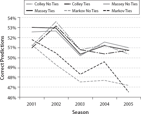
Colley, Massey, and Markov NHL foresight performance: ties vs. no ties

This graph does not point to a winner in the ties vs. no-ties debate.¹ We tested several other seasons of other sports, including basketball and football, and came to the following conclusion. While incorporating ties into a ranking method sometimes slightly improves the predictive performance, it rarely hurts. This rather lukewarm endorsement of ties prompted us to study the effect of induced ties, which are the subject of the next section and provide our most interesting finding in the ties vs. no-ties debate.

Induced Ties

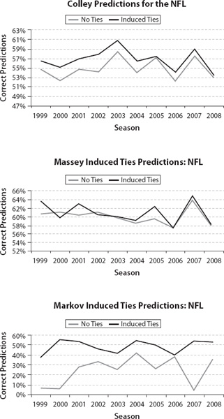
While some sports like hockey or soccer admit ties, other sports use overtime or sudden death rules to break ties that occur at the end of regulation time. In addition, there are some non-overtime events that appear to be won almost arbitrarily. The two teams are gridlocked in a tie or near tie for almost the entire game, then some last minute heroic breaks the tie. Basketball even has a phrase for such heroics—a “buzzer beater” refers to a shot that wins the game in the waning seconds. In such situations, it can be argued that a tie would be a more appropriate measure of the two teams’ strengths. Consequently, in this section, we induce ties in these instances and study the effect of our changes. For example, in NFL football we induce a tie for every game that ended with a final point differential of three or fewer points. The following three graphs show the effect of induced ties on the ten NFL seasons from 1999 to 2008 for the three ranking methods of Colley, Massey, and Markov. The previous three graphs show that the induction of ties clearly improves the predictive performance of these three ranking methods. The results were similar for the other ranking methods and other datasets such as college football.

We also studied the effect of induced ties in college basketball. While football has a rather obvious margin of victory for which to induce a tie (the 3 points scored by a field goal), basketball has a less obvious margin, so we varied the number of points required to induce a tie from 0 to 6. The results for the Colley method are shown below.

The no-ties results are the dashed line while all induced-ties methods are represented by solid lines. The solid lines vary in darkness from the light gray of the induced-ties method for the smallest margin of victory (one point) to the black of the largest margin of victory (6 points). Most margins of victory for the induced-ties methods outperform their no-ties versions. While it is hard to determine which margin of victory gives the best improvement in terms of the predictive performance, we do see a trend that the larger margins of victory generally outperform the lower margins of victory. We save a more precise study of the optimal margin of victory for inducing ties for future work.

In summary, the experiments of this section show that there is a clear winner in the ties vs. no-ties debate. The induced-ties method regularly outperforms the no-ties method as a predictive scoring measure.

Summary

Given the availability of large datasets in the modern world of computing and the frequent need to rank data, the fact that one may wish to use sports ranking methods in which input data may have ties, and the potential impact on incorporating ties into such results, one should carefully consider using methods that include ties. This chapter discussed how to include ties in several common ranking methods. Further, we introduced the idea of induced ties, which can improve the predictive performance of rankings.

Some questions remain. For example, what is the most effective way to induce ties for specific sports? Perhaps it makes sense to induce a tie in a low-scoring sport like soccer when the winning goal was scored in the last few minutes of regulation play. Of course, this raises the question of how many minutes should be viewed as “the last few” of a game. In basketball, a game can be close until the losing team begins fouling, hoping missed shots will reduce the margin of victory with little reduction in the time left in the game. You might ask if inducing ties in this context was beneficial and, presumably, how to automate such a decision among all games since making such decisions game by game is impractical. Other statistics could be also be analyzed—e.g., points per possession rather than score might be integrated in a ranking method and decisions regarding ties.

In addition, are there datasets where one expects ties to be less important? Are there datasets where one expects ties to affect certain locations in the ranking? For what other applications and methods are ties useful?

 

 

 

 

 

 

¹We dug deeper by examining the locations at which the two methods differed in their prediction and tried to determine if one method did a better job predicting at top-ranked positions, yet failed at lower-rank positions. However, this too drew no clear conclusion in the ties vs. no ties debate.