
Chapter Twelve
Incorporating Weights
“A preoccupation with the future not only prevents us from seeing the present as it is but often prompts us to rearrange the past.”—Eric Hoffer (1902–1983)
Rearranging the past is what this chapter is about. In fact, this is the first chapter that is more art than science. The art of ranking includes the ability to customize a method based on expert or application-specific information. Here’s a scenario: Team A lost two early-season games, then went undefeated for the remainder of the season, while team B was undefeated save for two late-season games. In your opinion, which team should be ranked higher? Most people say team A, since “preseason doesn’t matter.” That intuition sparked the mathematics of this chapter.
In all of the models presented thus far (with the possible exception of the Elo method), every matchup has been weighted equally. While at first blush, it sounds fair that no matchup carries more weight than another, this may not make sound modeling sense. For instance, in sports, shouldn’t end-of-season tournament games carry more weight than pre-season or early season games? Shouldn’t a team on a hot streak be more likely to win than a team on a cold streak? For webpages, perhaps pages that are updated more often should be more important. As a result, it’s natural to try to incorporate such time considerations into the models.
Weighting Ideas
While we emphasize weighting by time in this chapter, all sorts of weightings are possible. For example, one could weight wins at away locations more heavily than wins at home. Or one could weight wins against known rivals more heavily. That’s one feature of weightings—they are flexible enough to accommodate any weighting rationale you can dream up.
Four Basic Weighting Schemes
Weighting games is easy in most models. Though there are numerous possibilities and variations on the following, here we present four basic weighting schemes: linear, logarithmic, exponential, and step function weighting. To relay how easy and natural weighting is, we demonstrate weighting with the Markov model. In this case, the entries vij of the weighted Markov voting matrix ![]() are computed as
are computed as
![]()
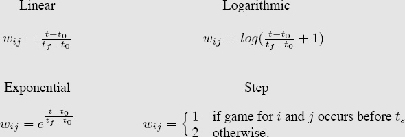
where wij is a scalar that accounts for the weight of the game played by teams i and j, and vij is the number of votes team i cast for team j (from the voting options for the Markov model of Chapter 6). The weight wij is determined by the weighting function. We propose four basic weighting functions, which are displayed in Figure 12.1 and described in turn below. Again, we talk specifically about time weightings, but any weighting or combination of weightings may be used.
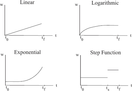
Figure 12.1 Four basic weighting functions
For a linear weighting scheme,
![]()
The numerator represents the time of the game relative to the season opener. Specifically, it is the number of days since the season opener, which occurred at time t0. The denominator is the total number of days in the season, which is given by the time of the season finale tf minus the time of the season opener t0.
If we want to weight later games in a slowly increasing manner, we use a logarithmic weighting scheme such as
![]()
On the other hand, if we want to dramatically exaggerate the weight of games at the end of the season, we use an exponential weighting scheme
![]()
The fourth weighting scheme that we describe in this chapter uses a step function. One possible step function weights games that occur in the last 2 (or 3 or 4 or k) weeks more than other games. One way to add extra weight to games occurring later in the season is to simply double (or triple or quadruple, etc.) count their corresponding votes. This works rather well, particularly for basketball as shown by the experiments of Luke Ingram’s M.S. thesis [41]. In this case,
![]()
where ts is some specific time during the season, such as one month prior to the conference tournament. Of course, a multi-step function could be implemented easily as well. This is precisely what Davidson College undergraduate Erich Kreutzer did for the 2009 March Madness tournament [19]. He created a step function that increased the weight of games every two weeks. His biweekly step function for the Colley method did so well that it got an ESPN score of 1420 (out of a total possible 1600) and was in the 97.3 percentile of all 4.6 million brackets submitted to the annual ESPN Tournament Challenge that year.
Summary of and Notation for the Time Weighting Schemes
wij weight given to matchup between teams i and j
t0 time of season opener (e.g., day 1 of season occurs when t0 = 0)
tf time of final game of season
ts specific time during season to change step weighting
t time of current game under consideration
Below are four simple methods for weighting a game between teams i and j that occurred at time t.
Now let’s discuss the details concerning how a weighting scheme can be applied to specific ranking methods.
Weighted Massey
For the Massey model, each game in a season is represented by a row in the original Massey linear system Xr = y. Each game and thus each row of the Massey system can be weighted according to its temporal occurrence in the season using any chosen weighting scheme. In this case, rather than solving Xr = y as a least squares problem, a weighted least squares problem is solved. First, a vector w of weights associated with each game is created. Again, perhaps games are weighted by their time from the beginning of the season so that late season games are more important. Next, w is transformed into a diagonal matrix W that has w along its diagonal. Finally, the weighted normal equations [36]
XTWXr = XTWy
are solved in order to produce the unique weighted least squares solution to the weighted original system W1/2Xr = W1/2y.
Weighted Colley
To weight the Colley method the off-diagonal elements of the Colley matrix C are no longer integers for the number of times teams faced each other, instead they are weights associated with the importance of each game. For example, in the unweighted context, if cij = 3, meaning teams i and j faced each other three times, then in the weighted context, cij is the sum of the weights associated with these three matchups. Similarly, the right-hand side vector b no longer contains a count of total wins minus total losses, instead it contains weighted counts. In terms of programming, this weighting modification is an easy adjustment to the algorithm.
Weighted Keener
Once a weighting method has been selected, the weighted Keener matrix ![]() is populated according to the formula
is populated according to the formula
![]()
where wij is the weight of the matchup between teams i and j and aij is the Keener statistic of choice from Chapter 4. Once this weighted Keener matrix is available, the remaining steps of the Keener method are executed as usual. Because nonnegativity of the Keener matrix is required, one must use nonnegative weights wij.
Weighted Elo
The K factor of the Elo method is the method’s built-in mechanism for weighting. Recall from Chapter 5 that for soccer the constant K is used to weight wins during World Cup finals (K = 60) more than World Cup qualifiers (K = 40) more than other tournaments (K = 30).
Weighted Markov
Once a weighting method has been selected, the weighted Markov voting matrix ![]() is populated according to the formula
is populated according to the formula
![]()
where wij is the weight of the matchup between teams i and j and vij is the number of votes team i cast for team j using one of the voting methods of Chapter 6. Once this weighted voting matrix is available, the remaining steps of the Markov model are executed without modification. That is, the weighted voting matrix ![]() is row normalized and, if necessary, a procedure for handling undefeated teams is applied. At this point, the stochastic Markov matrix S is available and the stationary vector, i.e., the rating vector r, is computed.
is row normalized and, if necessary, a procedure for handling undefeated teams is applied. At this point, the stochastic Markov matrix S is available and the stationary vector, i.e., the rating vector r, is computed.
Weighted OD
Weighting the OD method is nearly identical in implementation to the Markov method. That is, weighting is a preprocessing step to the OD method. Specifically, the elements pij of the OD P are massaged with the appropriate weighting scheme, then OD is computed as usual using this weighted P matrix.
Weighted Differential Methods
Time weighting can be incorporated easily into both the rank-differential and the rating-differential methods of Chapter 8. The actual algorithms do not change, only the input data matrix D changes as it is weighted before normalization according to the techniques discussed on page 147.
ASIDE: Weighting and the March Madness Tournament
Our work with weighting and the annual March Madness basketball tournament began in 2006 and has developed its own history in that time. Each year our weighting work gets more sophisticated as an outgoing group of researchers passes the torch to an incoming group. Here we chronicle the highlights of this work and introduce the main contributors.
• 2006: For a class project at the College of Charleston, then graduate students Luke Ingram and John McConnell were the first to tackle a March Madness prediction problem. Their goal was to use mathematical techniques to predict games in the tournament. The two discovered ESPN’s Tournament Challenge (and their $10,000 prize) and its online automated bracket submission and scoring tool. That year the pair submitted a few variants of the Markov model to ESPN. Because Luke and John believed momentum had strong predictive power, one submission used time-weighting to doubly count games in the month leading up to the tournament. Unfortunately, for Luke and John, whom other classmates had dubbed “The Apostles,” 2006 was the Year of the Upset. Many readers may remember the Cinderella run that the 11-seeded George Mason had, making it all the way to the final four. Only a very small crop of fans (mostly G.M. alumni) had George Mason advancing this far. In fact, the fan who did win the ESPN Tournament Challenge that year had mistakenly entered George Mason, meaning instead George Washington. After realizing his mistake, Russell Pleasant submitted his corrected G.W.-favored bracket. Luckily, he did not delete his G.M.-favored bracket from the contest, as that was the one that earned him the $10,000 prize that year.
• 2008: In the spring of 2008, I [A. L.] assigned the same project to seniors Neil Goodson and Colin Stephenson. These two sports fans and mathematics majors eagerly took up the torch, picking up where Luke and John left off. By the ESPN deadline, our class helped the pair submit over 30 brackets created from rankings of various weightings of the Colley, Massey, Markov, and OD methods. Neil and Colin studied their brackets well and discovered some newsworthy trends.
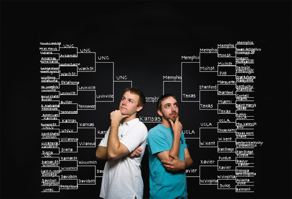
Figure 12.2 Neil Goodson and Colin Stephenson
For instance, most models predicted the dramatic upset of #11-seeded Kansas State over #6-seeded USC. Also, as most models predicted Kansas to win the whole tournament over Memphis, Neil and Colin decided to use the Massey method to predict the final score of a game between these two teams. Thus, they predicted Kansas to win in a very close game by just 3 points, a very good prediction given that Kansas won in overtime. The College of Charleston Media folks heard about Neil and Colin’s work and checked in regularly for updates as the tournament progressed. Propelled by their fantastic success in early rounds, Neil and Colin found themselves at the center of a media storm. Local media, including several newspaper and television stations, contacted the pair. Then came the national media, including an appearance on CBS’s The Early Show. Perhaps the most fame-inducing invitation came from Robert Siegel and his All Things Considered show on National Public Radio (NPR). Neil had a live phone interview during which he mentioned a few of his predictions, namely the big Kansas State upset and the champion Kansas University. Neil was a natural—striking just the right balance between the technical explanations of the mathematics and the exciting sports results and predictions. Neil’s segment received positive responses nationwide. In fact, he was so engaging that several nonsports listeners were so flabbergasted by the eventual accuracy of Neil’s prophesies that they felt compelled to call into the show after the tournament had ended. One listener called in to say that the pair did such a great job on their class project that their professor ought to give them an A. Their professor did—not for their spot-on predictions, but for their initiative and work ethic week after week all semester long. For more on the Neil and Colin story including one of their highest-scoring brackets, see the Aside on page 212.
• 2009: My [A. L.] Operations Research project class is offered only every other year at the College of Charleston. With the 2008 success fresh in mind, I certainly could not let this small fact inhibit our progress and 2009 March Madness fun. Thus, I teamed up with my good colleague, Dr. Tim Chartier of Davidson College, to run a cross-institutional ranking project. Our College of Charleston team consisted of graduate student Kathryn Pedings and undergraduate Ryan Parker. The Davidson team included Dr. Chartier and his undergraduate students Erich Kreutzer and Max Win. The overall team expanded to include Nick Dovidio, a Davidson alumni then at Stanford University, and Dr. Yoshitsugu Yamamoto of Tsukuba University, Japan. Our team truly spanned the country, continent, and globe as Figure 12.3 shows.
Kathryn Pedings
Yoshitsugu Yamamoto

Figure 12.3 Our March Madness team spans the globe
In 2009 we added a few more weightings as well as rankings from several rank-aggregation models (see Chapters 14 and 15). While 2009 was not quite as bracket-friendly as the historic and heralded 2008, we were very pleased with our progress. Several models scored in the 95th and 97th percentiles of all 4.6 million brackets submitted to the ESPN Challenge that year. And, once again, there was more press coverage, with articles in local newspapers.
• Each year our models grow in sophistication and whether or not a March Madness student ever claims the $10,000 ESPN prize, each student can claim mastery of essential hands-on modeling, programming, and communication skills, which have helped land some coveted job offers. In fact, Neil Goodson even heard the comment, “Hey, you’re that March Madness ranking guy from NPR, aren’t you?” on a job interview.