
Chapter Sixteen
Methods of Comparison
Chapters 2–8 presented a growing but finite set of methods for ranking items. When the weighting methods of Chapter 12 and the rank-aggregation methods of Chapters 14 and 15 are employed, the set of methods expands to a seemingly infinite set as the number of ways of combining these methods grows exponentially. Given this long list of possible methods for ranking items, a natural question arises: which ranking method (including the rank-aggregated methods) is best? In other words, how do we compare these methods for ranking items? As usual we begin our investigation by consulting the literature, which takes us back to the work of the statisticians Maurice Kendall and Charles Spearman.
Qualitative Deviation between Two Ranked Lists
Determining which ranked list is best among many is a very difficult problem, almost a holy grail. Yet there is a related question that is a bit easier to answer. That question asks how far apart any two ranked lists are. An answer to this question will eventually help us answer the more difficult question of which list is best. The topic of the numerical deviation1 between two ranked lists has been studied by statisticians and mathematicians for a while. In the sections on Kendall’s tau on page 203 and Spearman’s footrule on page 206 we describe two such classical numerical deviations and then add our own improvements to each.
While numerical deviations between two ranked lists give us a precise quantitative measure for comparing two lists, an imprecise qualitative assessment can also be useful at times. So before we delve into quantitative measures, we describe a visual display of the difference between two ranked lists.
Consider the two partial ranked lists l and ![]() of varying length below.
of varying length below.
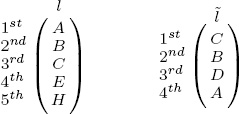
Figure 16.1 shows a bipartite graphical representation of the two lists.
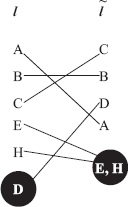
Figure 16.1 Bipartite graph comparison of two ranked lists
Because the lists are partial, there are some items, such as items D, E, and H, that appear in only one list. In order to handle such items, we insert one dummy node at the end of each ranked list and this node serves as a black hole. While we know which items belong in a black hole, we don’t know the relative order of items in each black hole. A line is used to connect each item on the left to its partner on the right. This graphical representation is a simple though powerful tool for assessing the difference in two ranked lists because horizontal or near horizontal lines mean that the two ranked lists have similar assessments of the quality of a particular item, whereas diagonal and steep diagonal lines mean the two lists had very dissimilar assessments about the position of the item. Further, a quick scan also reveals information about the location of the disagreements. For instance, many steep diagonal lines near the top of the bipartite graph means that the two lists disagreed strongly and often about top ranked items. If there are diagonal lines in the graph, we’d prefer that they occur towards the bottom of the graph. For example, Figure 16.2 shows the differences between the top-20 ranked lists produced by the Markov method and the Massey methods as compared to the RPI (Ratings Percentage Index) list. This calculation was done at the end of the 2005 NCAA men’s Division 1 basketball season. RPI is a recognized standard of the strength of a team and is one of the factors used by the NCAA to determine which teams are invited to the March Madness tournament. This line chart representation makes it easy to see that the Massey list has more in common with RPI than the Markov list.
An even more helpful visual display merges this bipartite graph with the number line representation of rating vectors. In this case, the first place and the last place teams are placed a fixed distance apart, then the remaining teams are positioned relative to their corresponding rating values. This shows the relative distances between teams. Each list is presented this way and teams are then connected creating a bipartite graph between the two lists. Figure 16.3 does this for the Massey and Markov rankings of Southern Conference teams for the 2007–2008 basketball season.
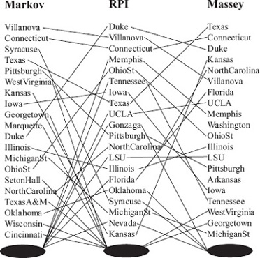
Figure 16.2 Bipartite graph comparison of Markov and RPI and Massey and RPI
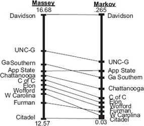
Figure 16.3 Bipartite plus line graph comparison of Massey and Markov methods
Kendall’s Tau
While the graphical representations of Figures 16.1 and 16.2 give a rough qualitative handle on the similarity of two ranked lists, quantitative measures add the missing precision. In this section we discuss a quantitative measure attributed to statistician Maurice Kendall. Kendall originally defined his measure for full lists and so some adjustment is required to make it apply to partial lists. Thus, we divide this section into those two cases, full lists and partial lists.
Kendall’s Tau on Full Lists
In 1938 Maurice Kendall developed a measure, today known as the Kendall tau rank correlation that determines the correlation between two full lists of equal size [43]. Kendall’s correlation measure τ gives the degree to which one list agrees (or disagrees) with another. In fact, one way to calculate part of the measure is to count the number of swaps needed by a bubble sort algorithm to permute one list to the other. However, the more common definition of Kendall’s τ is
![]()
where nc is the number of concordant pairs and nd is the number of discordant pairs. The denominator, n(n − 1)/2, is the total number of pairs of n items in the lists. For each pair of items in the list (i.e., each matchup), we determine if the relative rankings between the two lists match. More precisely, for pair (i, j), if team i is ranked above (or below) team j in both lists, then the pair is called concordant. Otherwise, it is discordant. The fractional representation of τ reveals its intuition as a measure of agreement between two lists. Since each of the n(n − 1)/2 pairs is labeled as either concordant or discordant, clearly, −1 ≤ τ ≤ 1. If τ = 1, then the two lists are in perfect agreement. If τ = −1, then one list is the complete reverse of the other.
EXAMPLE Consider the following three ranked lists l1, l2, and l3, which are full lists containing four items labeled A through D.
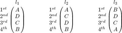
The measure between lists l1 and l2, denoted τ(l1, l2) is 4/6, while τ(l1, l3) = −4/6. This matches our intuition as it is easy to see that list l1 is closer to list l2 than it is to list l3. Further, list l3 is the reverse of l2 and so the Kendall distance τ(l2, l3) = −6/6 = −1.
The Kendall tau measure is a nice starting point for comparing the deviation between two ranked lists. However, it has a few drawbacks. First, it is expensive to compute when the lists are very long [28]. Second, both lists must be full, which limits the measure’s applicability. Often we want to compare so-called top-k lists. For example, we may want to compare the top-10 list of college football teams produced by the BCS with the top-10 list produced by one of our ranking methods. In this case, because the lists are partial, it is highly unlikely that the two lists will contain the same sets of teams. As a result, the standard Kendall measure cannot be used, though variants of it [25, 24, 47] have been proposed for such cases. In fact, we propose our own in the next section. Third, and particularly pertinent to our sports ranking problem, is the fact that disagreements occurring at the bottom of a ranked list incur the same penalties as disagreements at the top of the list. For most ranking applications, one is generally more concerned with elements toward the top of the ranked lists. In other words, errors at the bottom of the list are less important. This last weakness of the Kendall tau measure provided the motivation for the new distance measure proposed in in the section on Spearman’s footrule on 206.
Kendall’s Tau on Partial Lists
Kendall’s tau requires some adjustment in order to be applied to partial lists and lists of varying size. For example, consider lists l and ![]() below.
below.
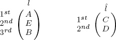
In this case, there are pairs of items, such as the (A,B) pair, for which there is not enough information to attach either the concordant or the discordant label. We need a new label, an unknown label for such pairs. In fact, in the above example, there are four such unlabeled pairs: (A,B), (A,E), (B,E), and (C,D). To accommodate this, we modify the Kendall tau measure for full lists to cover partial lists, including partial lists of varying size and lists containing ties.
![]()
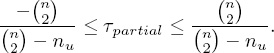
In the formula for τpartial, nc and nd are as usual (i.e., the number of concordant and discordant pairs respectively), n is the total number of unique items between the lists (i.e., |l ∪ ![]() |), and nu is the number of unlabeled pairs. For the above example,
|), and nu is the number of unlabeled pairs. For the above example,
![]()
which is the upper bound on the deviation for this example because
One advantage of τpartial is that it gives a higher penalty to disjoint partial lists than reverse partial lists, which agrees nicely with our intuition.
EXAMPLE Given the four partial lists below
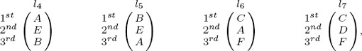
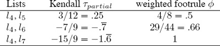
a straightforward application of this modified Kendall measure produces the values in Table 16.1. These values are rather unsettling for it appears that l6 is closer to l4 than l5 is, even
Table 16.1 Kendall τpartial with incorrect counting for n
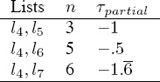
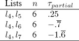
though l4 and l6 share just one common item. This example highlights a very important caveat of the τpartial measure—when comparing more than two partial lists, the counts for n, nc, nd, and nu only make sense when n is defined as the number of unique items among all lists in consideration. With this revision, τpartial agrees nicely with our intuition. Thus, for lists l4, l5, l6, and l7, n = 6 and the τpartial measures are given in Table 16.2.
Table 16.2 Kendall τpartial with correct counting for n
Notice that if full lists are used as input, then the number of unlabeled pairs is zero (i.e., nu = 0), so the τpartial formula (16.2) on page 205 collapses to the full τ formula (16.1) on page 204. Thus, the following definition suffices to cover both cases.
Kendall τ Measure for Comparing Ranked Lists
![]()
where nc is the number of concordant pairs, nd is the number of discordant pairs, nu is the number of unlabeled pairs, and n is the number of unique items among all lists being compared.
We have modified Kendall’s measure to accommodate both full and partial lists. This new modified definition also accommodates such special cases as partial lists of varying length and lists with ties. Yet one problem remains unsolved. Kendall’s τ uses simple counts (nd and nu) to penalize disagreements between lists. As a result, these penalties do not consider the relative position of such disagreements, which brings us to a new measure that weights disagreements according to their position in the list. After considering full lists, we will tackle the tougher case of partial lists.
Spearman’s Weighted Footrule on Full Lists
The new measure that we define in this section is a natural extension of an older measure, called the Spearman footrule measure, for comparing two ranked lists [41]. Spearman’s footrule ρ is simply the L1 distance between two sorted full lists l and ![]() of length k. That is,
of length k. That is,
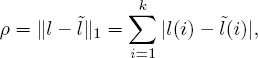
where l(i) is the ranking of team i in list l and ![]() (i) is the ranking of team i in list
(i) is the ranking of team i in list ![]() . Our modification is to weight the penalty associated with each discrepancy so that our new measure, which we call the weighted footrule, is defined in Equation 16.3.
. Our modification is to weight the penalty associated with each discrepancy so that our new measure, which we call the weighted footrule, is defined in Equation 16.3.
Weighted Footrule ![]() Measure for Comparing Two Full Ranked Lists
Measure for Comparing Two Full Ranked Lists
The weighted footrule measure ![]() between two full ranked lists l and
between two full ranked lists l and ![]() , both of length k, is
, both of length k, is
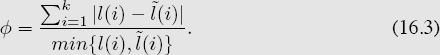
Notice that this new deviation measure is based on the following notion. Given two ranked lists, disagreements toward the top of the lists are more worrisome than disagreements toward the bottom of the lists. As a result, when computing a deviation measure, we penalize disagreements relative to their position in the list. This definition of ![]() heavily penalizes disagreements between high ranked teams.
heavily penalizes disagreements between high ranked teams.
EXAMPLE Suppose team i is ranked third in l and second in ![]() , then
, then
min{l(i), ![]() (i)} = 2,
(i)} = 2,
whereas if team i is 13th in l and 12th in ![]() , then min{l(i),
, then min{l(i), ![]() (i)} = 12, which results in a significantly reduced penalty
(i)} = 12, which results in a significantly reduced penalty ![]() for a disagreement that appears further down the top-k list.
for a disagreement that appears further down the top-k list.
Clearly, 1 ≤ min{l(i), ![]() (i)} ≤ k for all teams i that appear in both lists. Notice that
(i)} ≤ k for all teams i that appear in both lists. Notice that ![]() ≥ 0 so that the smaller
≥ 0 so that the smaller ![]() is, the closer the two lists being compared.
is, the closer the two lists being compared.
Spearman’s Weighted Footrule on Partial Lists
The weighted footrule is straightforward to calculate in the case of full lists. However, we must consider the more general (and more complicated case) of partial lists, which can be further subdivided into partial lists of equal length and partial lists of varying length. We begin with the easier case and consider two partial lists of length k.
The analysis of partial lists is tricky because an item may not appear in both lists. To calculate ![]() we must consider the contribution from each item i in the universe or union of items in both lists l and
we must consider the contribution from each item i in the universe or union of items in both lists l and ![]() . And each item i belongs either to the intersection l ∩
. And each item i belongs either to the intersection l ∩ ![]() (and thus appears in both lists) or the complement of this, (l ∪
(and thus appears in both lists) or the complement of this, (l ∪ ![]() )/(l ∩
)/(l ∩ ![]() ) (and thus appears in only one list). The contribution of
) (and thus appears in only one list). The contribution of ![]() i to
i to ![]() = ∑i
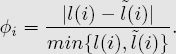
= ∑i![]() i for teams i in the intersection is easy to compute—simply use the weighted footrule Equation (16.3). However, the contribution for teams i in the complement is harder to calculate because exactly one of l(i) and
i for teams i in the intersection is easy to compute—simply use the weighted footrule Equation (16.3). However, the contribution for teams i in the complement is harder to calculate because exactly one of l(i) and ![]() (i) is unknown. Suppose, for example, that team i holds rank position j in list l but is absent from list
(i) is unknown. Suppose, for example, that team i holds rank position j in list l but is absent from list ![]() . Then
. Then ![]() i = |j −
i = |j − ![]() (i)|/j and
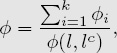
(i)|/j and ![]() (i) is obviously a missing piece of information. For now we will call this missing data x as it is an unknown quantity we hope to find eventually with the help of mathematical analysis. Thus, in the given scenario,
(i) is obviously a missing piece of information. For now we will call this missing data x as it is an unknown quantity we hope to find eventually with the help of mathematical analysis. Thus, in the given scenario, ![]() Once x is available we build our final deviation measure
Once x is available we build our final deviation measure ![]() by summing all the individual
by summing all the individual ![]() i penalties, i.e.,
i penalties, i.e., ![]() , where m is the total number of teams appearing between the two lists, i.e., m = |l(i) ∪
, where m is the total number of teams appearing between the two lists, i.e., m = |l(i) ∪ ![]() (i)|. The interpretation is simple: the smaller
(i)|. The interpretation is simple: the smaller ![]() is, the closer the two lists are.
is, the closer the two lists are.
Let us now fill in the missing piece of the puzzle associated with ![]() by finding the unknown x. We follow a mathematical analysis that is similar to the logic found in [47], which is based on the belief that a good measure
by finding the unknown x. We follow a mathematical analysis that is similar to the logic found in [47], which is based on the belief that a good measure ![]() ought to satisfy the following three properties.
ought to satisfy the following three properties.
1. Two identical lists should have a deviation measure of zero, i.e., ![]() = 0.
= 0.
2. Two disjoint lists should have the maximum deviation allowed by the measure.
3. The deviation between two lists whose elements are in exactly opposite order but whose intersections are full should be half of the deviation calculated in Property 2.
We use Properties 2 and 3 to cleverly determine x and thereby compute ![]() for partial lists of equal length.
for partial lists of equal length.
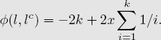
First, we begin with Property 2 and calculate ![]() (l, lc), the deviation between a list l and its disjoint partner lc. Since x is unknown, this computation will be a function of x. Assume l and lc are both of length k. Since l and lc have no common elements, there are 2k individual
(l, lc), the deviation between a list l and its disjoint partner lc. Since x is unknown, this computation will be a function of x. Assume l and lc are both of length k. Since l and lc have no common elements, there are 2k individual ![]() i measures to compute. For the first list l, the
i measures to compute. For the first list l, the ![]() i distances are
i distances are
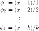
and the distances for list lc are identical. Thus,
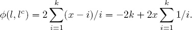
This sum, which depends on the values of k and x, is the maximum distance between two lists of length k. As a result, ![]() (l, lc) can also be used to normalize deviation values as a later final step. In summary, at this point, we have a value for Property 2, the maximum deviation allowed by the measure.
(l, lc) can also be used to normalize deviation values as a later final step. In summary, at this point, we have a value for Property 2, the maximum deviation allowed by the measure.
We now move onto Property 3 and compute ![]() (l, lr), the deviation between a list l and its reverse lr. The strategy is to obtain expressions for
(l, lr), the deviation between a list l and its reverse lr. The strategy is to obtain expressions for ![]() (l, lc) and
(l, lc) and ![]() (l, lr) in terms of k and x, then proceed by using the equation
(l, lr) in terms of k and x, then proceed by using the equation ![]() (l, lc) = 2
(l, lc) = 2![]() (l, lr) to solve for the unknown x.
(l, lr) to solve for the unknown x.
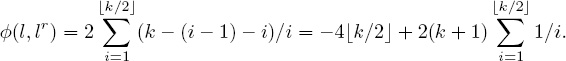
Since the list l and its reverse lr contain the same set of k items (i.e., l ∪ lr = l ∩ lr), ![]() (l, lr) will not be a function of the unknown x. As a consequence,
(l, lr) will not be a function of the unknown x. As a consequence, ![]() (l, lr) is a straightforward computation. We use the floor operator
(l, lr) is a straightforward computation. We use the floor operator ![]() to write
to write
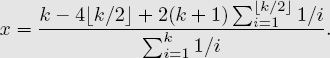
Finally, the last piece of the puzzle associated with x employs the equation ![]() (l, lc) = 2
(l, lc) = 2![]() (l, lr) to find an expression, though messy, for x. After a little algebra, we find (voila!)
(l, lr) to find an expression, though messy, for x. After a little algebra, we find (voila!)
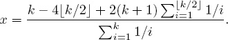
Thus, for example, for k = 3, ![]() (l, lc) = 8,
(l, lc) = 8, ![]() (l, lr) = 4, and x = 42/11 ≈ 3.82. Because normalized measures are easier to interpret, we force
(l, lr) = 4, and x = 42/11 ≈ 3.82. Because normalized measures are easier to interpret, we force ![]() to be between 0 and 1 by dividing by the maximum possible deviation, which is given by
to be between 0 and 1 by dividing by the maximum possible deviation, which is given by ![]() (l, lc).
(l, lc).
Weighted Footrule ![]() Measure for Comparing Partial Lists of Length k
Measure for Comparing Partial Lists of Length k
The weighted footrule measure ![]() between two length k partial lists l and
between two length k partial lists l and ![]() is built from individual
is built from individual ![]() i values and normalized so that 0 ≤
i values and normalized so that 0 ≤ ![]() ≤ 1. The closer
≤ 1. The closer ![]() is to its lower bound of 0, the closer the two ranked lists are.
is to its lower bound of 0, the closer the two ranked lists are.
where
Each item i belongs to one of the following two cases, and thus its contribution ![]() i to
i to ![]() is calculated accordingly.
is calculated accordingly.
• For item i ∈ l ∩ ![]() (i.e, an item appearing in both lists l and
(i.e, an item appearing in both lists l and ![]() ),
),
• For item i ∈ (l ∪ ![]() )/(l ∩
)/(l ∩ ![]() ) (i.e., an item appearing in only one list, which without loss of generality, we assume is l),
) (i.e., an item appearing in only one list, which without loss of generality, we assume is l),
![]()
where x is defined as
EXAMPLE Consider the four lists l4, l5, l6, and l7 from page 205, which are copied below.
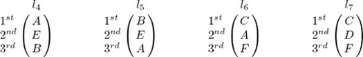
Table 16.3 shows the Kendall measure τpartial and the weighted footrule measure ![]() between list l4 and each other list. The differences in the two deviation measures are not as
between list l4 and each other list. The differences in the two deviation measures are not as
Table 16.3 Kendall tau and weighted footrule measures for four partial lists l4, l5, l6, and l7
apparent in this small example as they are in larger examples. In fact, the next example makes the differences between τ and ![]() very clear.
very clear.
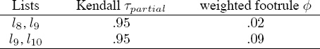
EXAMPLE Consider the example of Figure 16.4, which contains three lists l8, l9, and l10, all of length 12. Table 16.4 shows that τ(l8, l9) = τ(l9, l10) yet list l8 is certainly
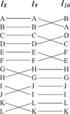
Figure 16.4 Difference between Kendall τ and weighted footrule ![]()
considered closer to l9 than l10 is because the top half of its rankings match those of l9 exactly. On the other hand, ![]() (l8, l9) <
(l8, l9) < ![]() (l9, l10) and the weighted footrule captures this preference.
(l9, l10) and the weighted footrule captures this preference.
Table 16.4 Kendall tau and weighted footrule measures for three partial lists l8, l9, l10
Partial Lists of Varying Length
The previous section showed that after performing some mathematical gymnastics, we could apply the weighted footrule measure to partial lists of equal length. Unfortunately, the gymnastics required to make ![]() applicable to partial lists of varying length are much more convoluted and thus are not justified. In practice, it is very rare to find an application that compares two lists of varying length. Contrast this limitation of the Kendall tau measure, which we were able to modify so that it could be applied to all lists: full lists, partial lists of equal length, and partial lists of varying size. On the other hand, the weighted footrule
applicable to partial lists of varying length are much more convoluted and thus are not justified. In practice, it is very rare to find an application that compares two lists of varying length. Contrast this limitation of the Kendall tau measure, which we were able to modify so that it could be applied to all lists: full lists, partial lists of equal length, and partial lists of varying size. On the other hand, the weighted footrule ![]() is more intuitive and appropriate than the Kendall τ for full lists and top-k lists as shown by the example with lists l8, l9, and l10.
is more intuitive and appropriate than the Kendall τ for full lists and top-k lists as shown by the example with lists l8, l9, and l10.
Yardsticks: Comparing to a Known Standard
Now that we have created a measure, ![]() , that we are very satisfied with for comparing two ranked lists (especially when they are of equal length), we return to the original question posed at the start of this chapter. That is, specifically which ranked list is best? There is a simple answer to this question when there is an agreed upon yardstick for measuring success. Consider once again the case of college football. Often the BCS ranked list is used as the yardstick for success. In this case, we compute
, that we are very satisfied with for comparing two ranked lists (especially when they are of equal length), we return to the original question posed at the start of this chapter. That is, specifically which ranked list is best? There is a simple answer to this question when there is an agreed upon yardstick for measuring success. Consider once again the case of college football. Often the BCS ranked list is used as the yardstick for success. In this case, we compute ![]() (BCS, Massey),
(BCS, Massey), ![]() (BCS, Colley), or
(BCS, Colley), or ![]() (BCS, Method), the deviation between BCS and any ranking method we desire. Then we simply declare the method creating the smallest
(BCS, Method), the deviation between BCS and any ranking method we desire. Then we simply declare the method creating the smallest ![]() as the best method. Of course, this presumes that the BCS list is “correct,” which, as we have pointed out previously, is a subject of perpetual debate. Because it is unsatisfying to hold a controversial ranked list such as the BCS as the gold standard, perhaps another list is more worthy of the golden status, which brings us to the next section.
as the best method. Of course, this presumes that the BCS list is “correct,” which, as we have pointed out previously, is a subject of perpetual debate. Because it is unsatisfying to hold a controversial ranked list such as the BCS as the gold standard, perhaps another list is more worthy of the golden status, which brings us to the next section.
Yardsticks: Comparing to an Aggregated List
A rank-aggregated list that is created using one of the aggregation methods of Chapter 14 seems like an excellent candidate for the gold standard or yardstick title. This list contains the best properties of many individual ranked lists and removes the effect of outliers. With this yardstick, we declare a ranked list as best if its deviation from the aggregated yardstick is smallest. Of course, either Kendall’s τ discussed on page 203 or the weighted footrule ![]() introduced on page 206 can be used to measure the deviation from the aggregated list.
introduced on page 206 can be used to measure the deviation from the aggregated list.
EXAMPLE Figure 16.5 shows the deviation from an aggregated list to the OD list and the Markov list. Both the qualitative and quantitative measures are provided. The bipartite graphical representation visually shows that the OD list is closer to the aggregated list than the Markov list is. This aggregated list was produced using the rating-aggregation method discussed in the section on rating aggregation on 176. The two numerical measures τ and ![]() then precisely quantify and reinforce this qualitative observation. Recall that, for the Kendall measure, the more positive τ is the more the lists agree. On the other hand, for the weighted footrule measure, a value of
then precisely quantify and reinforce this qualitative observation. Recall that, for the Kendall measure, the more positive τ is the more the lists agree. On the other hand, for the weighted footrule measure, a value of ![]() close to 0 means that the two lists agree often. In this example, which was taken from data for the 2004–2005 NCAA men’s basketball season, we’d declare the OD method as the superior method since it is closest to the aggregated list.
close to 0 means that the two lists agree often. In this example, which was taken from data for the 2004–2005 NCAA men’s basketball season, we’d declare the OD method as the superior method since it is closest to the aggregated list.
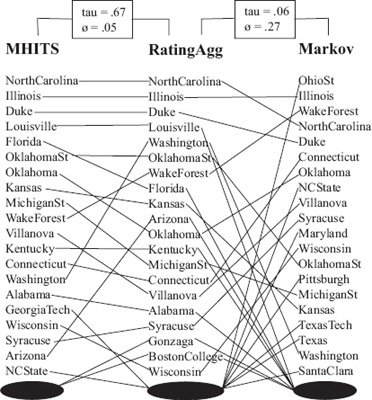
Figure 16.5 Comparison with distances between (OD, RatingAgg) and (Markov, RatingAgg)
Retroactive Scoring
Retroactive scoring uses a ranked list to predict the winners of past matchups. Based on this, various scores can be generated for a ranked list. For instance, every prediction that matches with past history may garner a ranking method one point. The method with the most points wins and is declared the best method for that year. The scoring can be more advanced if margins of victory are considered. For applications for which past matchup data is available, retroactive scoring presents a straightforward method for determining the quality of a ranked list.
Future Predictions
Future predictions are very similar in spirit to retroactive scoring. Except in this case, the quality of a ranked list is determined by its ability to predict the outcome of future games. The most common scenario here uses the ranked lists created at the end of a season to predict outcomes of end-of-year tournaments. As the next aside explains, the college basketball March Madness tournament is a perfect example.
ASIDE: Bracketology
Each the March NCAA Division I college basketball season culminates with a March Madness tournament. A set of teams are invited or obtain automatic bids to play in this end-of-the-season single elimination tournament. The tournament ends with the Final Championship game, which determines the year’s national champion. March Madness generates enormous fanfare in terms of press, betting, income, attention, road trips, and merchandise. One of the many ways fans can participate in the March Madness is through bracketology. Fans complete a tournament bracket before play officially begins. This entails selecting a team to win in each of the initial matchups, then following these outcomes to future matchups, selecting more winners, and continuing until a winner for each of the 65 matchups has been predicted. Fans can submit their brackets to office pools or even larger contests, including ESPN’s annual Tournament Challenge, in which the fan with the most accurate bracket wins $10,000. As the tournament progresses, correct predictions are given more weight. In fact, ESPN uses the following rules to tally scores for each submitted bracket: each correct prediction of a Round 1 game is worth 10 points, Round 2, 20 points, Round 3, 40 points, Round 4, 80 points, Round 5, 120 points, and Round 6, 160 points. A completely correct bracket scores the maximum of 1680 points. Below is an example of a bracket that Neil Goodson and Colin Stephenson, (two former College of Charleston undergraduate students) generated and submitted to ESPN’s contest for the 2008 tournament.
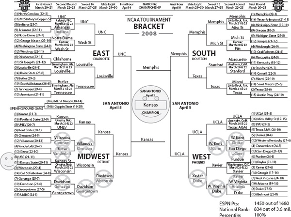
This bracket was produced from the ranking of the logarithmically weighted OD model of Chapter 7. To fill in predictions for a given matchup, the students compared the positions of the two teams in the ranking vector. The team with the higher rank was predicted to advance. When the tournament ended, Colin and Neil’s bracket received an ESPN score of 1450. Of the over 3.6 million brackets submitted, their bracket was in the 100th percentile at rank position 834. Incorrect predictions are denoted with an “X” in the bracket. And the two smiley faces indicate correct predictions that were upsets, i.e., most sports analysts did not have the predicted team advancing. The results of several other high-performing models from this book that were also submitted to the ESPN Challenge are listed in Table 16.5.
We are happy to report that Neil and Colin’s brackets did so well that they received a shocking amount of national press. The pair appeared on NPR’s “All Things Considered” and The CBS “Early Show.”
Table 16.5 Ranking Methods and ESPN scores for the 2008 tournament
Method |
ESPN score |
Massey Linear |
1450 |
Massey Log |
1450 |
OD Log |
1450 |
Massey Step |
1420 |
Massey Exponential |
1400 |
OD Step |
1320 |
Massey Uniform |
1310 |
OD Linear |
1310 |
OD Uniform |
1310 |
Colley Linear |
1100 |
Colley Log |
1010 |
Learning Curve
Yet another means of judging the quality of a ranked list concerns the intelligence of the ranking method that produced the corresponding list. A ranking method is considered “smart” if it requires a short warm-up period before it starts making correct predictions. Here’s a typical scenario. Each week of the NFL season, groups of friends form small-scale informal gambling operations to predict winners of that week’s matchups. Each week the participant with the most correct predictions wins the weekly pot. Of course, the ranking methods in this book could be used to predict winners. Yet in this scenario, to maximize earnings, the choice of a ranking method must consider both the method’s accuracy and its intelligence. A highly accurate method may require many weeks of data before its predictions outperform other methods, and thus, may not be the method garnering the highest payout. Anjela Govan, a Ph.D. student at North Carolina State University, conducted a similar operation (minus the money) as part of her doctoral dissertation [34].
Distance to Hillside Form
The last means for assessing the quality of a ranked list uses the reordering idea from Chapter 8. In this case, we use the ranking to symmetrically reorder a data differential matrix, such as the Markov point differential matrix V, and compute its distance from the hillside form defined on page 108. This distance can be measured with a (possibly weighted) count of the number of violations of the hillside constraints. The method producing the smallest number of violations is considered the best method.
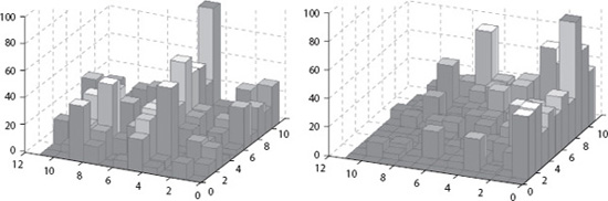
In fact, this is exactly what College of Charleston graduate student Kathryn Pedings did to compare a few ranking methods of the eleven 2007–2008 SoCon basketball teams. She found that, among the methods in Table 16.6, the reordering method called the rating-differential method produced a ranking with the minimum number of violations from hillside form.
This is not surprising as this method is an optimization problem designed to minimize this objective. Shown below is a cityplot view of the data-differential matrix with the teams in original order, then reordered according to the rating-differential method.
Table 16.6 Ranking methods and their number of violations from hillside form
Method |
# violations |
Rating Diff. |
265 |
OD |
268 |
Massey |
269 |
Colley |
275 |
$3,000,000, 000 ≤ total wagers on the NCAA men’s basketball tournament each year.
— More is bet on this event than on any other single U.S. sporting event.
— FBI estimates (Kvam & Sokol [48])
1Careful readers perhaps noticed that in this section we call our new measure ![]() a deviation, rather than a distance, measure. This is intentional. In order to be a distance measure
a deviation, rather than a distance, measure. This is intentional. In order to be a distance measure ![]() must satisfy the following three properties for all lists l1, l2, and l3.
must satisfy the following three properties for all lists l1, l2, and l3.
• The Identity Property: ![]() (l1, l2) = 0 if and only if l1 = l2,
(l1, l2) = 0 if and only if l1 = l2,
• The Symmetry Property: ![]() (l1, l2) =
(l1, l2) = ![]() (l2, l1), and
(l2, l1), and
• The Triangle Inequality: ![]() (l1, l2) +
(l1, l2) + ![]() (l2, l3) ≥
(l2, l3) ≥ ![]() (ll, l3) for all l1, l2, l3.
(ll, l3) for all l1, l2, l3.
Our measure ![]() passes the identity and symmetry properties yet fails the triangle inequality. Thus, we must settle with calling
passes the identity and symmetry properties yet fails the triangle inequality. Thus, we must settle with calling ![]() a deviation measure, and we are happy to do so, as this measure has been tailored to our particular sports ranking problem. In other words, its salient properties are more important to us than the triangle inequality.
a deviation measure, and we are happy to do so, as this measure has been tailored to our particular sports ranking problem. In other words, its salient properties are more important to us than the triangle inequality.