Chapter Ten

User Preference Ratings

The “spread rating” ideas that were introduced in (9.4) on page 120 transcend sports ratings and rankings. A major issue that has arisen in recent years in the wake of online commerce is that of rating and ranking items by user preference. While they may not have been the first to employ user rating and ranking systems for product recommendation, companies such as Amazon.com and Netflix have developed highly refined (and proprietary) techniques for online marketing based on product recommendation systems. It would require another book to delve into all of the details surrounding these technologies, but we can nevertheless hint at how some of the ideas surrounding the spread ratings might apply.

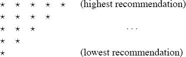
Suppose that we are an e-tailer selling products on the World Wide Web, and suppose that we collect user preference scores in a manner similar to Amazon.com—i.e., each product is scored by a user on a five-star scale.

The goal is to turn these user scores into a rating system that we can use to suggest highly rated products similar to the ones that the shopper is currently viewing or buying. It is not possible to effectively leaf through a large inventory catalog with a Web browser, especially if one is not sure of what they want or what’s in the catalog, so a large portion of the success of online retailing depends on the degree to which a company can be effective in recommending products that customers can trust. It’s simple,

Build a better product rating system Generate greater trust Make more sales!

Building a simple product rating system from user recommendations is easily accomplished just by reinterpreting the skew-symmetric score-differential matrix K on page 118. For example, suppose that

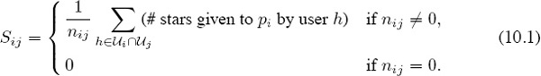
is the set of products in our inventory, and let _i and _j respectively denote the set of all users that have evaluated products p_i and p_j, so _i ∩ _j is the set of all users that have evaluated both of them. When comparing p_i and p_j (i ≠ j), let n_ij = #(_i ∩ _j) be the number of users that evaluate both of them, and define the “score” that p_i makes against p_j, to be the average star rating

Define, the “score difference” between products p_i and p_j to be

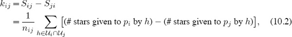
and, just as in (9.4), let

be the skew-symmetric matrix of score differences. The development on page 120 produces the following conclusion regarding the best ratings that can be produced by averaging a given set of “star scores.”

For example, suppose ten users = {h₁, h₂, . . . , h₁₀} have evaluated four products P = {p₁, p₂, p₃, p₄} using a five-star scale, and suppose that their individual evaluations (number of stars) are accumulated in the matrix

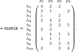
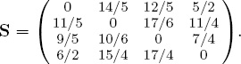
Notice that there are several missing entries in this matrix because not all users evaluate all products. In fact, the desire to extrapolate values for missing entries was the motivation behind the famous Netflix contest [56]. When the scores S_ij defined by (10.1) are arranged in a matrix, the resulting score matrix is

The skew-symmetric matrix K of score differences defined by (10.3) is

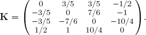
Therefore, the star ratings derived from user evaluations is

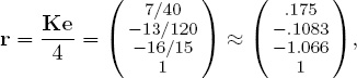
so the products rank (from highest to lowest) in the order {p₄, p₁, p₂, p₃}.

Direct Comparisons

Using the average star scores (10.2) to define the “score difference” between two products is a natural approach to adopt, but there are countless other ways to define score differences. For example, a retailer might be more interested in making direct product comparisons by setting S_ij to be the proportion of people in U_i ∩ U_j who prefer p_i over p_j. Such comparisons could be determined from user star scores if they were available, but direct comparisons are often obtained from old-fashion market surveys or point-of-sales data. To be precise, let

and define

If K is reinterpreted to be the skew-symmetric matrix of direct-comparison score differences

then the results in (9.4) on page 120 produce the following statement concerning the best “direct comparison” product ratings.

For example, suppose ten users U = {h₁, h₂, . . . , h₁₀} are involved in making direct comparisons of four products P = {p₁, p₂, p₃, p₄}, and suppose that the binary comparison results described in (10.4) are accumulated in the matrix

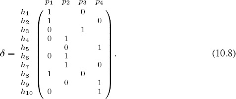
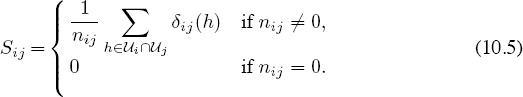
This means, for instance, that user h₁ compares products p₁ with p₃ and selects p₁, while user h₅ compares p₂ with p₄ and chooses p₄, etc. (The users need not be distinct—e.g., user h₁ could be the same as user h₅.) When the scores S_ij defined by (10.5) are arranged in a matrix, the resulting score matrix is

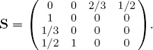
Consequently, the skew-symmetric matrix K of direct-comparison score differences is

and thus the direct-comparison product ratings derived from (10.7) is

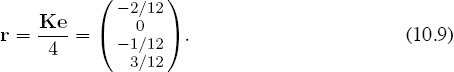
In other words, the products rank (from highest to lowest) in the order {p₄, p₂, p₃, p₁}.

Direct Comparisons, Preference Graphs, and Markov Chains

Another way to derive ratings based on direct comparisons between products is to build a preference graph. This is a directed graph with weighted edges in which the nodes of the graph represent the products in P = {p₁, p₂, . . . , p_n}, and a weighted edge from p_i to p_j represents, in some sense, the probability of favoring product p_j given that a person is currently “using” product p_i. While there are countless many ways to design user surveys to determine these probabilities, they can be constructed on the basis of direct comparisons such as those in the previous example (10.8).

1. For each product p_i, list all users H_i = {h_i1, h_i2, . . . , {h_i1, h_i2, . . . , h_ik,} who evaluated p_i.

2. If there is a user in H_i that prefers product p_j, then draw an edge from p_i to p_j.

3. The weight (or probability) q_ij associated with the edge from p_i to p_j is the proportion of users in H_i that prefer product p_j. In other words, if n_ij is the number of users in H_i that prefer product p_j. then

This preference graph defines a Markov chain [54, page 687], and rating the products in P can be accomplished by analyzing a random walk on this graph to determine the proportion of time spent at each node (or product). This is in essence the same procedure used in Chapter 6 on page 67. The idea is to mathematically watch a “random shopper” move forever from one product to another in the preference graph—if the shopper is currently at product p_i, then the shopper moves to product p_j with probability q_ij. The rating value r_i for product p_i is the proportion of time that the random shopper spends at that product.

If there is sufficient connectivity in the preference graph, then the proportion of time that a random shopper spends at product p_i (i.e., the rating value r_i) is the i^th component of the vector r that satisfies the equation.

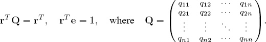
This vector r that defines our ratings is also called the stationary probability vector for the Markov chain (or random walk). This approach to rating and ranking is in fact the foundation of Google’s PageRank—see [49].

For example, consider the direct comparisons given in the matrix δ in (10.8) that are produced when ten users {h₁, h₂, . . . , h₁₀} evaluated four products {p₁, p₂, p₃, p₄}. From the data in δ we see that

p₁ is evaluated by users {h₁, h₂, h₃, h₄, h₆, h₈, h₁₀} = H₁,
p₂ is evaluated by users {h₄, h₅, h₆, h₇, h₉} = H₂,
p₃ is evaluated by users {h₁, h₃, h₈} = H₃,
p₄ is evaluated by users {h₂, h₅, h₇, h₉, h₁₀} = H₄.

Furthermore, we can also see from δ that of the seven users who evaluated p₁, three of them preferred p₁; two of them preferred p₂; two of them preferred p₃; and one of them preferred p₄. Consequently, there are four edges (paths) leaving node p₁ in the preference graph shown in Figure 10.1 with respective weights q₁₁ = 3/7; q₁₂ = 2/7; q₁₃ = 2/7; and q₁₄ = 1/7, and thus the first row of Q, shown below in (10.10), is determined. Similarly, the edges (paths) leaving the second node p₂ and the entries in the second row of Q are derived by observing that of the five users who evaluated p₂, none preferred p₁; three preferred p₂; none preferred p₃; and two preferred p₄, so q₂₁ = 0; q₂₂ = 3/5; q₂₃ = 0; and q₂₄ = 2/5.

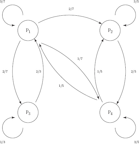
Figure 10.1 Product preference graph

Use the same reasoning to complete the preference graph and to generate the third and fourth rows of

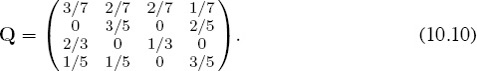
The Markov rating vector r is obtained by solving the five linear equations defined by

r^T (I − Q) = 0 and r^Te = 1

for the four unknowns {r₁, r₂, r₃, r₄}. The result is

so our four products are ranked (from highest to lowest) as {{p₄, p₂}, p₁, p₃}, where p₄and p₂ tied.

Centroids vs. Markov Chains

There are several problems with the Markov chain (or random walk) approach to rating. First, when there are a lot of states (or products in this case), there is often insufficient connectivity in the graph to ensure that the solution of r^TQ = r^T, r^T e = 1 (i.e., the ratings vector) is well defined. For such cases artificial information or perturbations must be somehow forced into the graph to overcome this problem, and this artificial information necessarily pollutes the purity of the “real” information—see [49]. Consequently, the resulting ratings and rankings are not true reflections of the actual data. However, this is a compromise that must be swallowed if Markov chains are to be used. On the other hand, using a centroid method requires no special structure in the data, so no artificial information need be introduced to produce ratings. Furthermore, even if the graph can be somehow perturbed or altered to guarantee that a well defined stationary probability vector exists, computing r can be a significant task in comparison to computing centroids, which is relatively trivial.

Conclusion

The centroid rankings (10.9) on page 130 and the Markov ratings (10.11) are both derived from the same direct comparisons data in (10.8). The centroid method ranks the products in the order {p₄, p₂, p₃, p₁}, while the Markov method yields the ranking as {{p₄, p₂}, p₁, p₃}. It is dangerous to draw conclusions from small artificial examples like these, but you can nevertheless see that the centroid rankings are in the same ball park as the Markov rankings. What is clear from this example is that the centroid rankings are significantly easier to determine, so if a centroid method can provide you with decent information, then they should be the method of choice.