
Chapter Fourteen
Rank Aggregation–Part 1
The dictum “the whole is greater than the sum of its parts” is the idea behind rank aggregation, which is the focus of this chapter and the next. The aim is to somehow merge several ranked lists in order build a single new superior ranked list.
The need for aggregating several ranked lists into one “super” list is common and has many applications. Consider, for instance, meta-search engines such as Excite, Hotbot, and Clusty that combine the ranked results from the major search engines into one (hopefully) superior ranked list. Figure 14.1 gives a pictorial representation of the concept of rank aggregation. Here l1, l2, . . . , lk represent k individual ranked lists that are somehow
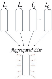
Figure 14.1 Rank aggregation of k ranked lists
combined, using mathematical techniques that will be explained in this chapter, to create one robust aggregated list. This process is called rank aggregation and has been studied extensively in [28], [25], and [24]. In fact, we have already encountered rank aggregation on page 82. There we needed to combine just two ranked lists, the offensive ranked list created by the OD rating vector o with the defensive ranked list created by the OD rating vector d. In that case, we used the simple rule r = o/d to create an aggregated rating vector r, which was then used to create the “robust” ranked list. In this chapter, we introduce several existing rank-aggregation methods that are more general in the sense that they can be used to combine any number of ranked lists. Then on pages 167 and 172 we introduce our contributions (two new algorithms) to the field of rank aggregation. However, before jumping into the methods we return once again to the topic that opened this book, political voting theory.
Arrow’s Criteria Revisited
This book began with a chapter on Arrow’s Impossibility Theorem [5], which states the limitations inherent in all voting systems. In summary, Arrow’s theorem says that no voting system can ever simultaneously satisfy the four criteria of an unrestricted domain, independence of irrelevant alternatives, the Pareto principle, and non-dictatorship. At least one of these criterion must be sacrificed. In this section we consider just how concerned we are with each criterion, especially given the particulars of the sports ranking problem.
While Chapter 1 pointed out the similarity between the problem of ranking candidates in a political system and the problem of ranking teams or individuals in sporting events, there are actually some differences between the two problems that are worth exploring in greater detail.
The context for Arrow’s theorem, i.e., political voting, differs from the sports ranking problem in two important respects. First, the political arena is mainly concerned with plurality voting. Creating ranked lists for all candidates is simply unnecessary because only the top ranked candidate has something to gain, whereas in sporting events such as volleyball, tennis, and NASCAR, first, second, third, and further place finishers typically receive points or cash prizes. Second, while political voting and sports ranking both have aspects of rank aggregation, the parameters in each case are quite different. Consider Figure 14.2, which shows the major differences in the data input and processing between the sports and political ranking problems.
Even if political elections asked voters to rank all candidates, there are relatively few candidates that run for most offices, while the pool of voters is huge. The situation is reversed in sports ranking, where typically only a handful of voters (ranking systems) rank hundreds of candidates (teams). And these two differences between the ranking systems, sports and politics, cause us to re-examine the justification for demanding that Arrow’s criteria hold.
Arrow’s first criterion requires that a voting system have an unrestricted domain, which means that every voter should be able to rank the candidates in any arrangement he or she desires. For instance, if the voting system required that an incumbent must be ranked in the top five, then Arrow’s first criterion would not be satisfied. In the sports ranking context, we agree with Arrow that an unrestricted domain is a desirable property.
On the other hand, Arrow’s second criterion, the independence of irrelevant alternatives, is probably the most controversial of Arrow’s demands on a voting system. It states that relative rankings within subsets of candidates should be maintained when expanding back to the whole set. Many voting theorists have debated the notion that society follows this axiom naturally, and the U.S. presidential election of 2000 highlighted for some the importance of this criterion. This dramatic election was so close that a winner could not be determined until the votes from the final submitting state of Florida were tallied. And even then recounts were issued as controversies concerning miscounts, chads, and the like surfaced. Many analysts speculated that Al Gore would have beaten George W. Bush in a head-to-head election in Florida if Ralph Nader had not taken some votes away from Gore. Votes cast for Nader allowed Bush to win what was essentially a best-out-of-three competition. In this case, Gore is what is known as the Condorcet winner and this situation is commonly referred to as the “spoiler effect” in the social choice literature. If the 2000 election had met Arrow’s independence criterion, then the rankings in the subset {Gore, Bush} should not have been affected by the advent of the third candidate in the expanded set {Gore, Bush, Nader}. The 2000 election showed that Condorcet winners can lose if a voting system does not satisfy Arrow’s second criterion.
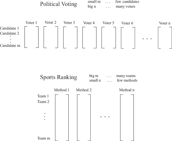
Figure 14.2 Differences in aggregating ranked lists in political voting vs. sports ranking
Since politics and sports are two quite different arenas, we now debate the relevancy of independence of irrelevant alternatives to our application of ranking sports teams. Nearly all sports rating methods use pair-wise matchups of teams. Note that “teams” can also be read as “candidates” to continue the comparison with political voting systems. We have already mentioned that for most sports, especially collegiate ones, a team does not face every other team during the season. There are just too many collegiate teams and not enough time to make this a realistic possibility. (Those scholar-athletes have to attend classes sometime.) Nevertheless, despite the fact that VT may never play USC during the season, we can still infer an indirect relationship between the two teams based upon inter-conference play. As a result, opponents of opponents can reveal once-removed connections between teams. That is, USC may have beaten UNC, who played and defeated VT. Thus, by the transitive property, one could argue that USC ought to be ranked above VT. Consequently, it can be argued that removing a team from a set of rankings should affect the overall rankings. And this statement leads us to reject Arrow’s second criterion for a rating system.
Yet another argument against the need for the independence of irrelevant alternatives can be made with the simple example of ranking wrestlers. It is common in many sports including wrestling, that j has an advantage over i in head-to-head matchups due to, for example, clashes in style. Yet j may be consistently defeated by most opponents while i performs very well against most opponents. As a result, wrestler i will perform very well in tournaments where he does not face j early on. When expanding to the set of all wrestlers in a tournament, i will almost always be ranked ahead of j after the tournament given that i and j did not wrestle in the first round. This is a violation of the independence criterion, which would require that j remain ranked ahead of i after expanding to the larger set of wrestlers. In summary, Arrow’s second criterion of the independence of irrelevant alternatives does not seem nearly as useful for the sports ranking problem as it does for the political voting problem.
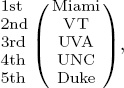
However, before we completely write off Arrow’s second criterion in the sports context, let us, for a moment, play the devil’s advocate and try to imagine a sporting scenario in which independence of alternatives is valuable. We use our running example to create just such a scenario. Recall from Table 1.1 that Miami, VT, UNC, and UVA all defeated Duke. A question that relates to the independence of irrelevant alternatives is: should the removal of Duke from Table 1.1 really affect the rankings? In other words, after the removal of Duke, should Miami’s rating be boosted more than UVA’s rating because Miami beat Duke by twenty more points than UVA beat Duke? Arrow would answer “No”, while the previous paragraph argued, “Yes, in some cases.” These are tricky questions. It is possible that, when facing Duke, a weak opponent, the UVA coach put in his second-string players, while Miami’s coach did not. Thus, perhaps a win over Duke should really carry very little weight, and thus, if Duke were removed from the set of candidates, then the rankings should be unaffected, which creates an argument in support of Arrow’s second criterion. Systems that incorporate game scores must reconcile the benefits of using point data with the problem of strong teams purposefully running up scores on weak teams. This “running up the score” issue appears to be the primary reason why the BCS prefers models that do not involve game scores, and instead only use win-loss records. Recall the bias-free notion embodied by the Colley method of Chapter 3. This scenario also highlights the fact that information regarding personnel changes or injuries is information that is not factored into any of the models in this book.
The above paragraphs present two ways of considering the independence criterion. In the first case, we presented an argument against it, and in the second case, an argument for it. Yet another way to examine this independence criterion is to take a mathematician’s perspective. Mathematicians often consider a model’s sensitivity to either small changes in the data or the prevalence of outliers. If a system gives stable results despite small changes in the input data, then the system is called robust, a desirable property. On the other hand, systems that are highly sensitive are undesirable. Consequently, it is natural to connect Arrow’s concept of independence of irrelevant alternatives with the mathematical notions of sensitivity and robustness. That is, a robust ranking method would satisfy Arrow’s second criterion.
There is much less debate over Arrow’s third criterion of the Pareto principle, which states that if all voters choose candidate A over B, then a proper voting system should maintain this order. This is clearly a desirable criterion to satisfy in both the political voting context and the sports ranking context. For example, if all methods rank Miami ahead of Duke, then an aggregated ranking of these methods should have Miami ranked ahead of Duke.
Arrow’s fourth and final criterion is non-dictatorship. While it seems obvious that no voter should have more weight than another in the political setting, this is not so obvious in the sports ranking context for two reasons. First, some of the aggregation techniques discussed in the next section require a “tie-breaking” strategy between lists of close proximity. In this case, usually one list is given priority over another by the aggregation function. Thus, the list given priority acts as a dictator or at least a partial dictator. In a second scenario, there may be a justifiable reason to have a (partial) dictator. For example, sports analysts may want to have rankings generated by coaches and experts count more (or less) than rankings generated by computer models. Such wishes can be accommodated if we are willing to break Arrow’s fourth criterion. As a result, it appears that Arrow’s final criterion is not as useful in the sports ranking context as it is in the political voting context.
Rank-Aggregation Methods
The idea of rank aggregation is not new. As the previous section implied, it has been studied for decades in the context of political voting theory. However, the field of web search brought renewed interest in rank aggregation. With the dramatic increase in the past decade of spamming techniques that aim to deceive search engines and achieve unjustly high rankings for client webpages, search engines needed to devise anti-spam counter methods. And this is precisely why and when rank-aggregation methods received renewed attention. For example, meta-search engines are based on the idea that aggregating the ranked lists produced by several search engines creates one super parent list that inherits the best properties of the child lists. Thus, if one child list from, say, Google contains an outlier (a page that has been successfully optimized by its owner to spam Google into giving it a very high though unjust ranking), then, after the rank aggregation, the effect of this outlier, this anomaly, should be mitigated. As a result, rank aggregation tends to act as a “smoother,” meaning that it removes any anomalous bumps or outliers in the rankings of individual lists and smoothes the results. Another property of a rank-aggregated list is that it is only as good (or as bad) as the lists from which it is built. That is, one cannot expect to create an extremely accurate rank-aggregated list given a set of poor input lists. In this section, we present four methods of rank aggregation. The first two are historically common ones, while the last two are our new contributions to the field of rank aggregation.
ASIDE: Web Spam and Meta-search Engines
This aside emphasizes the prevalence and pervasiveness of web spam by discussing two popular spamming techniques, Google bombs and link farms [49]. By the end, the need for spam-resistant rating methods will be clear. Fortunately, meta-search engines, which use rank-aggregation methods, such as the ones discussed in this chapter, have been successful at deterring spam.
A Google bomb is a spamming technique that exploits the high importance that Google places on anchor text. Perhaps the most famous Google bomb was aimed at G. W. Bush. Figure 14.3 shows the mechanism behind the bomb. The effectiveness of a Google bomb is tied to Google’s belief that the anchor text associated with a hyperlink serves as a short summary or synopsis of the webpage it points to. If several pages (in the example of Figure 14.3, Bob’s page, Jim’s blog, and Kim’s blog) all point to Bush’s White House biography page and carry the same anchor text of “miserable failure,” then Google assumes that Bush’s page must be about this topic. When enough spammers collude, this spamming strategy causes the target page, i.e., Bush’s page, to rank highly for the search phrase, i.e., “miserable failure.” When Google went public in 2004, their IPO documentation cited such spamming as a risk that investors must consider. The rank-aggregation techniques of this chapter offer one remedy to Google bombs. A meta-search engine that aggregates results from several major engines would find Google’s results for spammed phrases such as “miserable failure” to be inconsistent with the results from other search engines. The effect of these outliers would be mitigated by the rank-aggregation processes described in the next few sections.
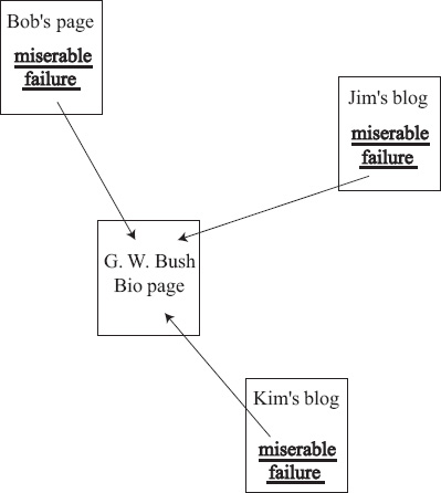
Figure 14.3 How a Google bomb works
A second popular spamming technique is the link farm. A link farm affects any search engine that incorporates link-based analysis into its ranking of webpages. Most link analysis algorithms, particularly Google and its PageRank algorithm, reward pages that receive inlinks from other high ranking pages. A link farm creates high ranking pages on general topics, then shares this PageRank with client pages. For example, consider Figure 14.4. A search engine optimization (SEO) firm may create a densely connected group of pages on topics such as former U.S. presidents. These pages contain valid relevant information on these topics and thus receive decent rankings from a search engine. When a customer contacts a SEO firm hoping to boost the rank of its page, a link is simply made from the link farm to the client’s page. Thus, in effect, the link farm was artificially created in order to share its PageRank with clients. Link farms are hard for search engines to detect and thus are a troublesome spamming technique. Just as in the case of Google bombs, one possible way to combat link farms is to employ the rank-aggregation techniques discussed in the next few sections.
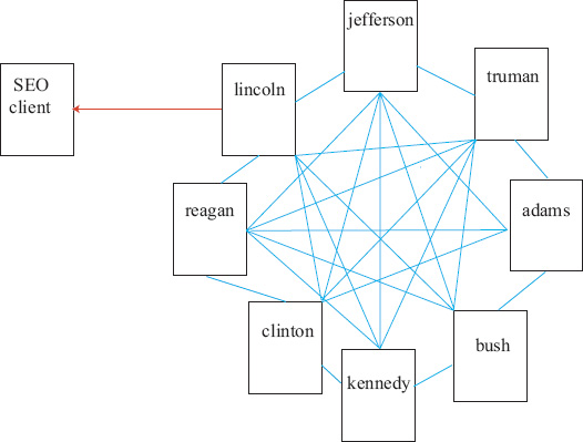
Figure 14.4 How a link farm works
Borda Count
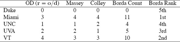
A common rank-aggregation technique is Borda’s method [12], which dates back to 1770 and Jean-Charles de Borda. Borda was trying to aggregate ranked lists of candidates from a political election. For each ranked list, each candidate receives a score that is equal to the number of candidates he or she outranks. The scores from each list are summed for each candidate to create a single number, which is called the Borda count. The candidates are ranked in descending order based on their Borda count. The BCS ranking method discussed in the aside on page 17 is popular example of how Borda counts are applied.
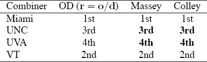
Though Borda’s method is very simple, an example provides the best, most concise explanation. And so we refer once again to our running 5-team example. Choosing the Borda count as the method for aggregating the three ranked lists from OD, Massey, and Colley, Table 14.1 lists the items needed for this computation. The number 4 listed next to VT in the OD column means that there were four teams that VT outranked in the OD list. By summing the rows for the three methods, we have a Borda count aggregation of the three lists.1
This example demonstrates the simplicity and computational ease associated with the Borda method for rank aggregation. In addition, the Borda count method of rank aggregation can be adapted to handle ties. For example, suppose a voter ranked the five teams from best to worst as {Miami, VT, UNC/UVA, Duke}, where the slash (/) indicates a tie. In this case, the Borda scores for this list are
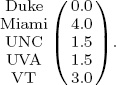
Table 14.1 Borda count method for aggregating rankings from OD, Massey, and Colley for 5-team example
Notice that teams that tie split the Borda scores of the fixed rank positions. Thus, the Borda count method can handle input lists with ties. In addition, though unlikely, the Borda count method could produce an output aggregate list that contains ties.
Unfortunately, the Borda method has one serious drawback in that it is easily manipulated. That is, dishonest voters can purposefully collude to skew the results in their favor. Textbooks, such as [16], provide classic examples demonstrating the manipulability of the Borda count.
ASIDE: Llull’s Count

This chapter presents the mathematical ideas of the Borda count and the Condorcet winner, which both take the namesake of their inventors. However, recently discovered manuscripts reveal that these mathematical ideas really ought to be called Llull counts and Llull winners after Ramon Llull (1232-1315), the extremely prolific Catalan writer, philosopher, theologian, astrologer, and missionary. Llull has over 250 written documents to his name. In 2001, with the discovery of three lost manuscripts, Ars notandi, Ars eleccionis and Alia ars eleccionis, historians discovered that they could add three more works to that tally and also add mathematician to Llull’s list of occupations and titles. Since Llull’s work on election theory predated Borda’s and Condorcet’s independent discoveries by several centuries, he has since been acknowledged as the first to discover the Borda count method described in this section and the Condorcet winner discussed on page 160.
Average Rank
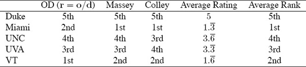
Another very simple rank-aggregation technique is average rank. In this case, the integers representing rank in several rank-ordered lists are averaged to create a rank-aggregated list. Again, an example makes this quite clear. Table 14.2 shows the average rank for the three ranked lists created by the OD, Massey, and Colley methods.
This example hides one drawback common to average rank—the frequent occurrence of ties in the average rating score. Let l1 and l2 be two full ranked lists. A full ranked list contains an arrangement of all elements in the set. Suppose team i is ranked first in l1, but third in l2, and team j is ranked second in both lists. In this case, average rank produces a tie for second place. To further complicate matters average rank can produce multi-way ties at multiple positions.
Table 14.2 Average rank method of aggregating rankings from OD, Massey, and Colley for the 5-team example
There are several strategies for breaking ties such as the one mentioned in the previous paragraph. We describe two. The first strategy makes use of past data to break ties. If teams i and j played each other, then the winner of that matchup (or the “best of” winner of multiple matchups) should be ranked ahead of the losing team. Retroactively using game outcomes to determine a tie-breaking team is more difficult when averaging more than two lists because several difficulties can arise. For example, suppose that teams i, j, and k tie for a rank position when three or more ranked lists are averaged. It is possible that the data used to create the lists contains the following outcomes: i defeated j, j defeated k, and k defeated i. This type of circular tie is a frequently cited difficulty with rankings created by pair-wise matchups. A typical solution is to assign one list as the tie-breaker list, which is a strategy described in the next paragraph.
If the teams involved in the tie never played, then the second tie-breaking strategy is to assign one ranked list as the “tie-breaking list,” which works well in the case of pair-wise ties. For example, suppose a tie scenario occurs in which teams i and j both vie for second position in the aggregated list. Yet suppose that the first ranked list has been chosen as the superior, and thus, tie-breaking list. Then this means that team i wins the second place position in the aggregated list and team j fills in the third position. The choice of tie-breaker list need not be arbitrary either, particularly if we have a method for determining which ranked list is better. Measures for determining the quality of a ranked list are discussed in Chapter 16.
We close this section with some observations regarding the average rank method of aggregation. First, note that average rank can be applied only if all lists are full (i.e., the intersection of the elements in all lists contains all teams). Second, the average rank method of aggregation can produce an aggregated list that does not contain ranks. This was clear from Table 14.2. Of course, the solution there was easy. The result of averaging ranked lists produces an average rating vector, which can then be transformed into a ranking vector.
Simulated Game Data
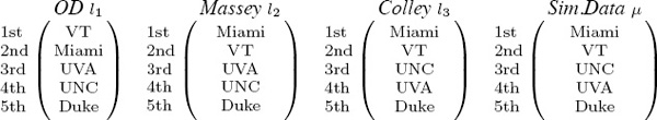
In this section we present a new rank-aggregation method that is born from a simple interpretation of a ranked list. See Figure 14.5. The interpretation is this: if team A appears above team B in a ranked list, then in a matchup between these two teams A ought to beat B. Further, if team A appears at the top of the ranked list and plays team B, which appears at the bottom of the list, then we expect A to beat B by a large margin of victory. The observation that a ranked list gives implicit information about future game outcomes seems rather natural. And yet the clever part, in terms of the mathematical modeling, is that we use ranked lists to generate so-called simulated game data, which we eventually use to aggregate the results of several lists into one list. In fact, each ranked list of length n provides data for ![]() = n(n − 1)/2 simulated games. Let’s return again to our 5-team example and the three ranked lists of OD, Massey, and Colley, which appear below.
= n(n − 1)/2 simulated games. Let’s return again to our 5-team example and the three ranked lists of OD, Massey, and Colley, which appear below.
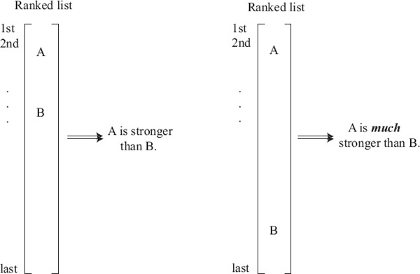
Figure 14.5 Interpretation of relative position of items in a ranked list
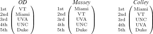
Starting with the OD ranking vector, we can form ![]() = 10 pair-wise matchups between these five teams. If VT played Miami, we’d expect VT to win, based on the information in the OD vector. Further, we can assign a margin of victory to this simulated game, if we simply assume that margins are related to the difference in the ranked positions of the two teams. This is where we, as modelers, have lots of wiggle room for creative ideas. Here we present one elementary idea that works well. We assign a margin of victory of one point for each difference in the rank positions. Thus, according to the OD vector, VT would beat Miami by one point, UVA by 2 points, UNC by 3 points, and Duke by 4 points. This point score data is useful later in the rank-aggregation step. After we have generated simulated game data for the OD ranking vector, we move onto the next ranking vector, and so on, until we have accumulated a mound of simulated game data. Note that any number of ranked lists can be used to build the complete set of simulated data. In the above example, with three ranked lists of five teams each, we generate
= 10 pair-wise matchups between these five teams. If VT played Miami, we’d expect VT to win, based on the information in the OD vector. Further, we can assign a margin of victory to this simulated game, if we simply assume that margins are related to the difference in the ranked positions of the two teams. This is where we, as modelers, have lots of wiggle room for creative ideas. Here we present one elementary idea that works well. We assign a margin of victory of one point for each difference in the rank positions. Thus, according to the OD vector, VT would beat Miami by one point, UVA by 2 points, UNC by 3 points, and Duke by 4 points. This point score data is useful later in the rank-aggregation step. After we have generated simulated game data for the OD ranking vector, we move onto the next ranking vector, and so on, until we have accumulated a mound of simulated game data. Note that any number of ranked lists can be used to build the complete set of simulated data. In the above example, with three ranked lists of five teams each, we generate ![]() simulated games. We also note that, unlike most other aggregation methods, the lists need not be full. Some lists may be full, some partial, and the simulated game data can be built nonetheless.
simulated games. We also note that, unlike most other aggregation methods, the lists need not be full. Some lists may be full, some partial, and the simulated game data can be built nonetheless.
Once the simulated data has been generated completely, the aggregation actually occurs in the next step, which we describe now. At this step, any ranking method is applied to the simulated game data. This ranking method, which we call the combiner method, could be an entirely different method. For instance, a method not used to create the input ranking vectors could be applied. Or on the other hand, a favored method from those used as input can be applied as the combiner method. In this case, that favored popular method, which has been used as both an input method and a combiner method, becomes in some sense a partial dictator, using Arrow’s language.
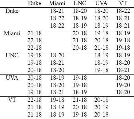
Table 14.3 shows the simulated game data built from the OD, Massey, and Colley ranking vectors. Notice that we have set the losing team’s score to 18. We could have chosen 0, 10, or any other arbitrary number (more wiggle room for experimentalists), yet since 18 was the average losing team’s score for the 2005 season, this is reasonable. Notice also that each cell of the 5 × 5 table contains three game outcomes, one for each of the three ranking vectors used as input. In particular, the 18-21 entry in the (Duke, Miami) cell indicates that in the OD ranking vector Duke appeared three rank positions below Miami and thus loses in a simulated matchup by three points. The 18-22 entry in that same cell comes from the Massey ranking vector, which had Duke four rank positions below Miami.
Table 14.3 simulated game data
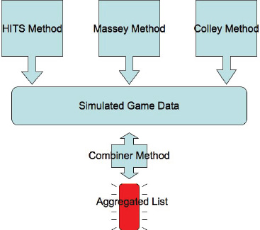
Simulated data method for rank aggregation
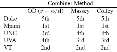
The diagram shown above gives a pictorial summary of the simulated data approach to rank aggregation. This approach is then used to aggregate the data from the OD, Massey, and Colley vectors for the small 5-team example. Table 14.4 shows that the aggregated results can differ slightly depending on the combiner method used.
Table 14.4 Simulated data method of rank aggregation using OD, Massey, and Colley as the combiner method
We point out four properties of the simulated data approach to rank aggregation.
• The rank-aggregated list is only as good (or as bad) as the input lists.
• The combiner method acts as a “smoother” in that it minimizes the effect of outliers, which are lists containing anomalies that seem inconsistent with the rankings in other lists. This comment whispers once again of Arrow’s second criterion, the independence of irrelevant alternatives, and the related issues of robustness and sensitivity. As an example of the impact of the combiner method, consider Table 14.4. To test for independence, we removed Duke from the data set, which forces a swap in the rankings between UNC and UVA when the Massey and Colley methods are used as the combiner methods. Compare Table 14.5 with Table 14.4. In contrast, using OD as the combiner method, creates a consistent ranking that is unaffected by the removal of Duke, the weakest team. Consequently, for this very small example, we say that the OD rank-aggregation method is robust.
Table 14.5 Simulated data method of rank aggregation and its sensitivity to the removal of Duke
• Rank-aggregated lists satisfy Arrow’s third criterion, the Pareto principle, so long as the input lists satisfy the Pareto principle.
• Though it is a small example, Table 14.4 shows that the combiner method can have an effect on the aggregated list. In addition, if the combiner method is also one of the input methods, then this method can be called a partial dictator in the language of Arrow’s fourth criterion.
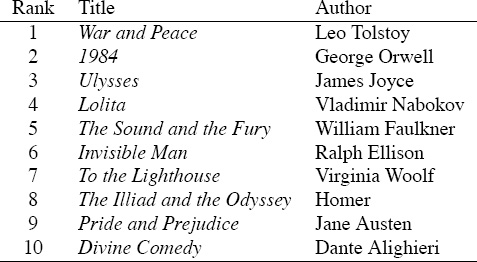
ASIDE: Top 10 Books—Aggregating Human-generated Lists
Most lists of the best books of all time are human-generated. In other words, surveys are conducted and votes are tallied. Book clubs, publishers, magazines, and the like each produce their top-10 lists of the best books ever. In June 2009 Newsweek produced their meta-list of the top-100 books. That is, they gathered ten top-10 lists from sources such as Time, Oprah’s Book Club, Wikipedia, and the New York Public Library and aggregated these lists to create their top-100 meta-list. Newsweek used a simple weighted voting scheme to aggregate these lists, but of course, they could have applied any of the rank-aggregation methods in this chapter (or the next) instead. For all the book-loving readers, the top-10 books of all time, according to Newsweek’s meta-list, are shown in Table 14.6
Table 14.6 Top-10 books of all-time according to Newsweek’s meta-list
Graph Theory Method of Rank Aggregation
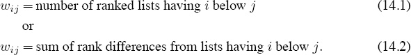
In this section we propose yet another method for aggregating several ranked lists. This method relies on graph theory. Consider the graph of Figure 14.6 below in which each team is a node in the graph. The weights are not game scores or, for that matter, any other statistical game data. Instead, the weights on the links in Figure 14.6 come from information in the ranked lists that we want to aggregate. For example, consider the following two suggestions for attaching a weight wij to the link from i to j.
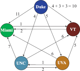
Figure 14.6 Graph for graph theory approach to rank aggregation for the 5-team example
The weights can be considered votes that weak teams cast for strong teams. These are just two possible ways to cast votes.
The discussion on page 176 explores an extension called rating aggregation that creates weights in the aggregated graph from the numerical values in the rating rather than the ranking vectors.
Once an approach for attaching weights to the links in the dense team graph has been selected, a favorite node ranking algorithm can be applied to this weighted graph. For instance, any of the popular node ranking algorithms from web search including PageRank, HITS, or SALSA, can be used. See [49] for more information on these algorithms.
We applied the PageRank method (a popular method for ranking nodes) [15] to the graph of Figure 14.6. This graph was built from the three ranking vectors displayed on p. 168 that were created by OD, Massey, and Colley. The links from Figure 14.6 are weighted according to Definition (14.2). For example, the link from Duke to VT has a weight of 4 + 3 + 3 = 10 because Duke appears 4 rank positions below VT in the OD vector, 3 rank positions below VT in the Massey vector, and 3 rank positions below VT in the Colley vector. Applying the PageRank method to this graph gives a PageRank vector that creates an aggregated ranking vector of
Graph theory aggregated ranking
which, by the way, matches the aggregated vector from Table 14.4 on p. 170 created from the simulated data method when Massey or Colley were used as the combiner method.
The two new rank-aggregation methods on pages 167 and 172 are much more sophisticated than the standard and existing methods discussed on pages 165 and 166. In fact, any serious rank-aggregation application, including college football’s hotly contested BCS rankings, should adopt one of these more advanced methods for aggregating the results of many ranked lists. Further, the next chapter presents an even more mathematically advanced method for rank aggregation, one that guarantees that the aggregated list optimally agrees with the input lists. See Chapter 15 for more on this aggregation method.
ASIDE: Rank Aggregation and Meta-search Engines
A meta-search engine combines the results from several search engines to produce its own ranked list for a particular query. In this aside, we demonstrate how a meta-search engine could use the graph theory method of rank aggregation presented in this section. First, we gathered four top-10 ranked lists by entering the query “rank aggregation” into the four search engines of Google, Yahoo, MSN-bing, and Ask.com. The union of these four lists contains n = 17 distinct webpages. Applying the graph theory method results in the aggregation matrix W of size 17 × 17. The PageRank vector of this graph produces the rank-aggregated list of webpages shown on page 174 that contains the results of our meta-search engine.
To implement the simple meta-search engine, proceed as follows.
1. Get the top-k lists from your p favorite search engines.
2. Create an aggregated matrix W using techniques described on page 172 (or any of the rank-aggregation techniques of this chapter or the next). The dimension of W is n × n where n is the number of distinct webpages in the union of the p lists.
3. Compute the ranking vector r associated with W.
Because k and p are typically small (k < 200, p < 10), W is small, and r can be computed in real-time.
Results of our simple meta-search engine for query of “rank aggregation”
A Refinement Step after Rank Aggregation
After several lists l1, l2, . . . , lk have been aggregated into one list μ using one of the procedures from the section on rank aggregation on page 163, a refinement step called local Kemenization [25] can be implemented to further improve the list μ. An aggregated list μ is said to be locally Kemeny optimal if there exist no pair-wise swaps of items in the list that will reduce the sum of Kendall tau measures between each input list li and μ where i = 1, . . . , k and μ. (The Kendall tau measure τ is carefully defined on page 203). For now it is enough to know that τ measures how far apart the ranked lists are.) Thus, the local Kemenization step considers each pair in μ and asks the question: will a swap improve the aggregated Kendall measure? An example serves to explain this refinement process. Consider the three input lists created from the OD (l1), Massey (l2), and Colley (l3) methods applied to the 5-team example along with the aggregated list (μ) from the simulated data aggregation technique on page 167.
The local Kemenization procedure begins with the highest ranked item (Miami) in the aggregated list µ and asks the question: does its neighboring item (VT) beat it (Miami) in the majority of the input lists? If yes, swap the two items as this creates a refined aggregated list with reduced Kendall distance. The same question is asked of each neighboring pair in the sorted aggregated list. Thus, for an aggregated list of length n, local Kemenization requires n − 1 checks, one for each neighboring pair.
LOCAL KEMENIZATION ON THE 5-TEAM EXAMPLE
Check #1
Question: Does the second place item (VT) beat the first place item (Miami) in the majority of the input lists?
Answer: No, VT beats Miami only once in the three input lists.
Action: None.
Check #2
Question: Does the third place item (UNC) beat the second place item (VT) in the majority of the input lists?
Answer: No, UNC never beats VT in the three input lists.
Action: None.
Check #3
Question: Does the fourth place item (UVA) beat the third place item (UNC) in the majority of the input lists?
Answer: Yes, UVA beats UNC in two out of three input lists.
Action: Swap UNC and UVA in µ.
Check #4
Question: Does the fifth place item (Duke) beat the fourth place item (UVA) in the majority of the input lists?
Answer: No, Duke never beats UVA in the three input lists.
Action: None.
Thus, the locally Kemenized aggregated list ![]() is
is 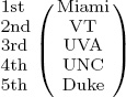 , which agrees with the aggregated lists produced by the Massey combined simulated data method and the Colley combined simulated data method shown in Table 14.4 on page 170.
Rating Aggregation
So far this chapter has taken up the issue of aggregating ranked lists, but of course each ranked list is derived from a rating list, which prompts the question: can rating lists be aggregated as well? The answer is yes, though there are some hurdles to jump. For instance, one hurdle concerns scale. How do we aggregate rating vectors when each contains numerical values of such differing scale? Recall that the Colley method produces ratings that hover around .5, while Markov produces positive ratings between 0 and 1. Even more complicated, some ratings, such as Massey ratings, contain positive and negative values. Figure 14.7 shows the number line representations for the rating vectors produced by the three methods that we will consider in this section: Massey, Colley, and OD. Notice the differing scales. In order to put such varying ratings on the same scale, we invoke distances
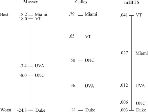
Figure 14.7 Number line representations for Massey, Colley, and OD vectors for the 5-team example
and percentages. A rating vector of length n actually contains ![]() = n(n −1)/2 pair-wise comparisons between the n total teams. Consider the Massey rating vector, rMassey, below.
= n(n −1)/2 pair-wise comparisons between the n total teams. Consider the Massey rating vector, rMassey, below.
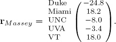
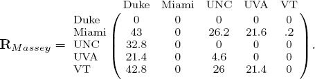
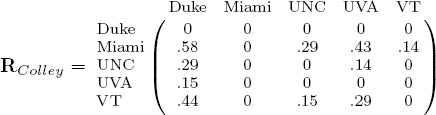
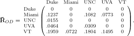
Because the rating for Miami is larger than that for Duke, the Massey method predicts Miami to beat Duke. Yet the difference between these two ratings, 43, is relatively large. Surely, this must mean something. In fact, we like to think of these rating differences as distances. Miami and Duke are very far apart while UNC and UVA, whose relative distance is 4.6, are close. Because it is natural to think of distances as positive, we can take differences in such a way to create an asymmetric nonnegative matrix of rating differences for each rating vector. For example, the Massey rating vector rMassey above produces the rating distance matrix RMassey below.
Computing rating distance matrices from the Colley and OD rating vectors produces
and
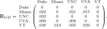
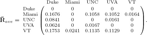
A quick glance at these R matrices demonstrates the problem of scale. In order to put these distances on the same scale we use the age-old trick of normalization. We divide each element of a raw R matrix by the sum of all distances in that matrix. The normalized matrices, denoted ![]() , are below.
, are below.
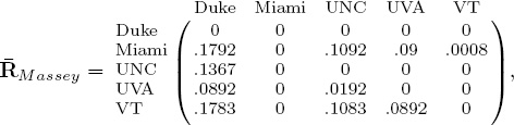
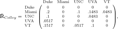
The interpretation of the .1792 element in the (Miami, Duke)-entry of the normalized ![]() Massey matrix is that the distance between Miami and Duke is 17.92% of the total distance predicted between all pair-wise matchups in the Massey model. The great advantage here is that percentages are measures that can be compared across different methods. Further, and more to the point of this section, ratings can now be aggregated. A simple rating aggregation method takes the (possibly weighted) average of several normalized
Massey matrix is that the distance between Miami and Duke is 17.92% of the total distance predicted between all pair-wise matchups in the Massey model. The great advantage here is that percentages are measures that can be compared across different methods. Further, and more to the point of this section, ratings can now be aggregated. A simple rating aggregation method takes the (possibly weighted) average of several normalized ![]() matrices. For example, averaging the normalized
matrices. For example, averaging the normalized ![]() Massey,
Massey, ![]() Colley, and
Colley, and ![]() OD produces
OD produces
Producing Rating Vectors from Rating Aggregation-Matrices
Each nonzero entry of matrix ![]() ave gives information about the distance between two teams, and thus, predictions about potential winners in future matchups. And with just a bit more work it may be possible to squeeze even more information out of
ave gives information about the distance between two teams, and thus, predictions about potential winners in future matchups. And with just a bit more work it may be possible to squeeze even more information out of ![]() ave to produce point spread predictions, the subject of future work. For now, we discuss methods for collapsing the information in the two-dimensional matrix into a one-dimensional rating vector. We present three methods for creating a rating vector r from
ave to produce point spread predictions, the subject of future work. For now, we discuss methods for collapsing the information in the two-dimensional matrix into a one-dimensional rating vector. We present three methods for creating a rating vector r from ![]() ave.
ave.
Method 1
The first method uses row and column sums. The row sums of ![]() ave give a measure of a team’s offensive output while the column sums give a measure of a team’s defensive output. That is, the offensive rating vector is o =
ave give a measure of a team’s offensive output while the column sums give a measure of a team’s defensive output. That is, the offensive rating vector is o = ![]() avee and the defensive rating vector is d = eT
avee and the defensive rating vector is d = eT ![]() ave, where e is the vector of all ones. Just like the OD model of Chapter 7, a high row sum corresponds to an effective offensive team and a low column sum corresponds to an effective defensive team. Thus, the overall rating vector for a team can be computed as r = o/d.
ave, where e is the vector of all ones. Just like the OD model of Chapter 7, a high row sum corresponds to an effective offensive team and a low column sum corresponds to an effective defensive team. Thus, the overall rating vector for a team can be computed as r = o/d.
Method 2
The second method for extracting a rating vector r from the ![]() ave matrix applies the Markov method to a row-normalized version of
ave matrix applies the Markov method to a row-normalized version of ![]() Tave. This works because the entries of
Tave. This works because the entries of ![]() ave are the distances between teams, or in other words, votes that one team casts for another.
ave are the distances between teams, or in other words, votes that one team casts for another.
Method 3
The third and final method for extracting a rating vector r from the matrix ![]() ave uses the dominant eigenvector of
ave uses the dominant eigenvector of ![]() ave. This eigenvector actually has a name—it is the Perron vector of
ave. This eigenvector actually has a name—it is the Perron vector of ![]() ave. This vector gets its name from the Perron theorem which tells us that the dominant eigenvector of an irreducible nonnegative matrix is guaranteed to be nonnegative. Rather than checking that
ave. This vector gets its name from the Perron theorem which tells us that the dominant eigenvector of an irreducible nonnegative matrix is guaranteed to be nonnegative. Rather than checking that ![]() ave is irreducible, in practice one can force irreducibility by adding ε eeT to
ave is irreducible, in practice one can force irreducibility by adding ε eeT to ![]() ave, where ε is a small positive scalar.
ave, where ε is a small positive scalar.
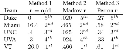
Table 14.7 shows the results of applying these three methods to create three rating vectors associated with ![]() ave.
ave.
Table 14.7 Rating vectors for three methods of rating aggregation
ASIDE: Ranking NSF Proposals
The National Science Foundation (NSF) is America’s largest funding agency for scientific work. As such, each year this governmental agency receives thousands of proposals from scientists each pitching their own research. Of course, the NSF budget, though large, is finite. As a result, decisions are continually being made as to which proposals to fund and which to reject. Most funding decisions are made with a procedure known as a panel review, which relies on the service of recognized experts in the field under consideration. For example, the NSF FODAVA (Foundations of Data and Visual Analytics) division may receive 32 proposals for the 2009 year. Approximately 20 panel reviewers (i.e., FODAVA experts who have little or no conflicts of interest with the proposers) are asked to read this collection of proposals. Because the volume of proposals makes it unrealistic for each panelist to read each proposal, division directors allocate roughly the same number of proposals to each panelist. For instance, most panelists are asked to review six proposals and some seven. Generally the directors like to have each proposal reviewed by at least three or four panelists. A panelist’s review consists of written comments plus, most relevant to this book, a rating. Ratings are Excellent, Very Good, Good, Fair, and Poor. Since not every proposal is read by every panelist and since some panelists may be generous in their ratings while others are more demanding, the system faces some inherent challenges. To combat such challenges, the NSF requires the panelists to assemble in a two-day face-to-face meeting wherein each proposal is summarized by those who reviewed it and then discussed by the entire panel. This discussion process is essential to the review process yet it is very time-consuming. Below we suggest one way to make these two-day meetings more efficient. The idea is to fairly aggregate the ratings so that one overall global ranked list can be produced. With such an aggregated list, less discussion time can be spent on the bottom, say, one-half of the proposals for which the panel collectively agrees should not be funded.
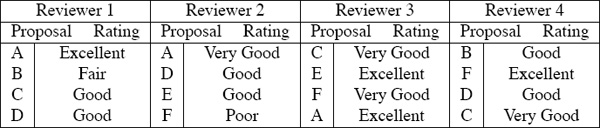
Let’s consider an example. Suppose there are six proposals labeled A through F that must be ranked and four reviewers who are each assigned four proposals to read. A typical panel session begins with the list of Table 14.8. This list nicely compiles reviewer ratings, yet it hides some important information concerning which reviewers gave which ratings. In fact, the list in Table 14.8 was actually produced from the information in Table 14.9, which clarifies the fact that reviewers use different scales to grade proposals. One reviewer (e.g., in this case, reviewer 2) may be very generous and give a high score of Very Good or Excellent liberally, whereas another may be much stingier and rarely if ever give out an Excellent. As a result, we use the ideas discussed in the section on rating aggregation on 176 to put the ratings of different reviewers on the same scale. Applying the rating-aggregation method produces the following ![]() matrices for the four reviewers.
matrices for the four reviewers.
Table 14.8 Proposal ratings for a sample NSF panel
Proposal |
Rating |
A |
Excellent, Very Good, Excellent |
B |
Fair, Good |
C |
Good, Very Good, Very Good |
D |
Good, Good, Good |
E |
Good, Excellent |
F |
Poor, Very Good, Excellent |
Table 14.9 Proposal ratings from each reviewer
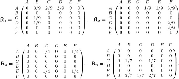
The numerator of the (A,B)-entry of ![]() 1 means that reviewer 1 rated proposal A three positions above proposal B. The denominator, 9, is the cumulative rating differentials of all
1 means that reviewer 1 rated proposal A three positions above proposal B. The denominator, 9, is the cumulative rating differentials of all ![]() possible matchups between proposals rated by reviewer 1. Averaging
possible matchups between proposals rated by reviewer 1. Averaging ![]() 1,
1, ![]() 2,
2, ![]() 3, and
3, and ![]() 4 creates the average distance matrix
4 creates the average distance matrix
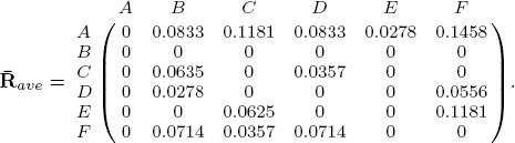
We used the third method from the section on rating aggregation on 178 to create a rating vector from ![]() ave. That is, we computed the Perron vector of
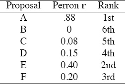
ave. That is, we computed the Perron vector of ![]() ave and arrived at the rating and ranking vectors appearing in Table 14.10. With these results, the panel might decide to discuss only A, E, and F as these are the top three according to the rating-aggregation method.
ave and arrived at the rating and ranking vectors appearing in Table 14.10. With these results, the panel might decide to discuss only A, E, and F as these are the top three according to the rating-aggregation method.
Table 14.10 Rating-aggregation method applied to NSF proposal example
Summary of Aggregation Methods
• The examples in this chapter demonstrated the use of aggregation methods by combining several computer-generated lists. However, these aggregation methods could also be used to combine human-generated lists or even merge data from both human and computer sources. Consequently, we see great potential for aggregation methods.
• While we have yet to prove a theorem with the following statement, our experiments have led us to posit that Qworst ≤ Qaggregate ≤ Qbest, where Q is a quality measure that can be used to score each method. (Part of the problem with proving such a statement lies in the design of an appropriate quality measure Q, which is a non-trivial matter. See Chapter 16.) The statement claims that an aggregated list may be outperformed by the lists produced by one or more individual methods. On the other hand, the aggregated list outperforms the lists produced by several other individual methods. Thus the aggregated list is helpful in one-time predictive situations.
ASIDE: March Madness Advice
Consider the annual March Madness tournament and its Bracket Challenge. Predicting a single event is tough and can be hit or miss. The individual (unaggregated) methods in this book predict well “on average,” i.e., over the course of many matchups between the same teams. Yet the Bracket Challenge requires that methods predict well in many single occurrence events. This “one-time” prediction problem is different from the “on average” or “best of” prediction problem. In particular, in “one-time” events, upsets are often more frequent due to the heightened, high-stakes circumstances associated with “one and done” style tournaments such as March Madness. Consequently, rather than banking on one particular method, if you must submit one and only one bracket, a wise (and more conservative) choice is to bet on an aggregate of several methods, which is precisely where the rank-aggregation methods of this chapter excel.
By The Numbers —
47,000,000,000 ≈ number of Web pages Google has rated and ranked
12,000,000,000 ≈ number of Web pages Yahoo! has rated and ranked
11,000,000,000 ≈ number of Web pages Bing has rated and ranked
— as of September 2011.
— worldwidewebsize.com
1We thank Luke Ingram for the creation of this data and table.