
Simulation of textile machinery
Abstract:
The simulation of textile machines is of increasing importance as trials of machines are often time consuming and expensive. In addition, many customers today demand quick production of small lots which in turn requires an optimized machine setting within a very short period of time. A wide range of methods is described in this chapter, covering processes from yarn production and processing through fabric manufacturing to finishing. The relevant systems of equations are explained where possible and simulation results are illustrated for selected examples of typical applications that have, in many cases, have been commercialized.
9.1 Introduction: simulation methods to optimize machine settings and product quality
The importance of developing mathematical models and simulation programs for textile machines becomes apparent when considering the following developments in recent years.
• Trials to run machines with new materials or new settings are increasingly time-consuming and expensive due to the ever-increasing complexity of textile machines.
• A lot of knowledge about proper machine settings is being lost due to many experienced textile workers retiring in developed countries where textile industries are longest established; workers in the developing world often lack the respective expertise and are thus not able to fill this gap.
• Customers expecting delivery of their orders within a very short period of time and ordering smaller lots in shorter intervals, thus not leaving enough time for time-consuming trials.
• Machines becoming faster which in turn increases wear on machine parts; this makes it ever more important to calculate optimum machine setting in order to reduce the stresses on the machine and its components to increase their economic life.
Developing simulation programs for textile machines requires both a profound mathematical and technical understanding of textile processes and textile materials as well as access to industrial-scale production facilities in order to verify the developed tools. Up until the turn of the millennium, these requirements were comparatively easy to meet in the industrialized world. Since then, the developing world has been gaining ground and it is to be expected that more and more computer simulations of textile machines will also be developed there in the years to come. So far, most simulations of textile machines that have been put into practice have been developed in Europe and this research thus predominates among the references at the end of this chapter. In the following sections, a range of mathematical models are presented, covering textile production from spinning through fabric production to finishing. Some selected examples, which have been put into practice or may in other ways be interesting for practical application, are described in detail.
Most simulation tools developed in recent years to improve machine settings for new materials, new products or new components use a numerical approach. They apply the methods described in the previous chapters such as artificial neural networks, evolutionary algorithms, fuzzy logic and computational fluid dynamics. The majority of models are based on data gathered through trials rather than on equations derived from the laws of physics. Only a very few published models apply the latter principle. Some of them are described in Section 9.2. In general, it is not difficult to optimize machine settings as the values by which the degree of optimization is assessed can normally be measured directly on the machine. This is not possible when it comes to improving product quality.
It has proven to be extremely difficult to relate product properties to machine settings via analytical equation systems for two reasons.
• Firstly, there are many parameters that have an influence on the final product quality that cannot be measured directly on a particular machine since several machines are normally employed to manufacture the final product.
• Secondly, and as a consequence of the first reason, there are a large number of parameters that influence each other or whose influence cannot be directly measured, e.g. yarn orientation, temperature, fineness and evenness of intermediate products. This makes it extremely complicated to include them all properly into a mathematical model.
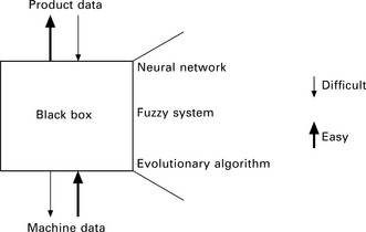
Hence, when it comes to improve the quality of products by applying simulation techniques, the vast majority of models that have been put into industrial practice are based on numerical methods as described in Chapters 2–5. As Fig. 9.1 shows, these models can principally work in both directions: predicting product quality based on the machine settings and optimizing machine settings to achieve certain product properties. Since a certain machine setting should always lead to a certain product quality, whereas a certain product quality can be achieved potentially with different machine settings, the first approach is much easier to be put into practice than the latter, as has already been explained in Chapter 2. Nevertheless, there are a few noteworthy examples of analytical approaches to improve product quality which are explained in the next section.
In this chapter, typical examples for the simulation of textile machines are described. They cover yarn formation, fabric production, finishing and plant design. Since there is often a direct industrial application of the results of such simulations, there are a number of mathematical models that have been developed by researchers directly for use in the textile industry. Since these were not published, they are not cited here.
9.2 Simulating yarn production and processing: ring/rotor spinning and false-twist texturing
Basligil (1994) published an extensive literature review with regard to papers on machine interference, explaining the basic concepts of machine interference and naming possible solutions. This is not a true simulation but nevertheless provides a valuable source for further information about this topic which could be used to create a mathematical model. An early example of mathematically modelling staple-fibre spinning processes can be found in Crank and Whitmore (1953, 1954) and Crank (1953). In these studies the effect of balloon height, cap radius, bobbin radius and speed and yarn fineness on, for example, the size of the balloon and on the yarn tension within the bobbin are analysed. Certain simplifying assumptions are made, e.g. that the cross-section of the yarn is circular and the thread itself perfectly flexible and inextensible. With this model, it was possible to determine conditions under which a balloon can develop or the yarn breaks due to high tension. The model itself is convincing, but experimental data to verify the results of the model were not given.
More recent papers about models to analyse balloon formation during ring-spinning include Batra et al. (1989a, 1989b). They showed that it is possible in principle to calculate, for example, the mass of the traveller required to achieve a certain yarn tension, the tension distribution along the yarn path and to determine the shape of the balloon. Data from actual trials to verify the model are not given.
Owing to increasing computer power, papers with more sophisticated mathematical models on ring spinning have been published. A typical example which is described below in more detail is Tang et al. (2010a). They designed a mathematical model and a numerical simulation to analyse dynamic behaviour and twist distribution in a modified ring spinning system which is shown in Fig. 9.2. In general, we have

9.2 Schematic diagram of a modified ring spinning system. (adapted from Tang et al., 2010a)
where m stands for the yarn fineness, ω denotes the angular velocity of the pin, ez coincides with the axis z in Fig. 9.3 and R(s, t) is the yarn path with s representing the arc length and t the time.

9.3 The balloon from the hook to the yarn guide. (adapted from Tang et al., 2010a)
The twist propagation equation according to Tang et al. (2010b) is given by
where N(s, t) stands for the rotation angle of the cross-section of the yarn at position s at point-in-time t and V0 represents the propagation velocity of the yarn twist, for which we have
with G, I and J representing the shear modulus, the polar moment of inertia and the unit moment of inertia.
In general, in ring spinning, it can be assumed that the twist propagation speed is much larger than the delivery speed of the yarn. The twist in each zone (see Fig. 9.2) then consists of three components: the original twist wave and the two waves coming from each adjacent boundary zone. At the winding point, we have
This model was used to create a computer simulation to predict the shape of the balloon and the tension along the yarn path from roller (Fig. 9.2, A) to the winding point at the bobbin (E). A typical bobbin curve is shown in Fig 9.3. Typical calculated results for the course of the yarn path are shown in Fig. 9.4 for different yarn tensions T0 at the yarn guide (C). These results were compared with yarn curves measured on an actual ring spinning machine and it was proven that the results coincide quantitatively. The calculated and the measured yarn twists were found to be very similar in all zones except CD. This was, according to the authors, due to the negligence of the yarn twist blockage of the yarn guide in the mathematical model. It remains to be seen whether a mathematical model of balloon formation will eventually also include this most interesting zone.
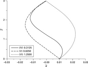
9.4 Typical bobbin curve. (adapted from Tang et al, 2010a)
Zhu and Wang (2011) tried to detect the origins of faults caused by rollers in a spinning machine. They used an improved wavelet technique to first extract the relevant frequencies and then to determine the cause of the fault. Four different causes were identified using this approach.
An unusual approach to optimize the output of an open end (OE)-rotor spinning machine was published by Braccesi and Carfagni (1993). In automated OE-rotor spinning machines, a robot moves along the machine and removes full bobbins, reattaches broken yarns, cleans spin boxes, etc. in this paper, a mathematical model was designed that simulates the resulting output of the machine depending on different behaviours of the robot. Figure 9.5 shows the general approach. It was found that the factor with the highest influence on the machine output (e.g. number of full bobbins) was the number of attempts the robot was allowed to try to fix a problem before moving on and leaving it to the operator to fix. Normally, a robot is allowed to try three times before resuming its movement along the machine with success rates in the range of 85%, 11% and 2% for the first, second and third attempts respectively. Allowing only one attempt does significantly increase the machine efficiency when the number of yarn breaks exceeds a certain limit, as can be seen in Fig. 9.6. The increase is more significant for coarse yarns than for thin yarns as the time needed to fix a problem relative to production time is directly correlated to the yarn fineness. Even if the success rate drops to 75% for the first attempt, this result persists.

9.5 Block diagram of the simulation. (adapted from Braccesi and Carfagni, 1993)

9.6 Machine output depending on no. of attempts to fix the problem. (adapted from Braccesi and Carfagni, 1993)
The simulation model thus showed that in order to achieve optimized robot settings, the number of yarn breaks and the yarn fineness should be taken into account in order to increase the machine output. Whereas shorter yarn reattachment and bobbin removal times have a direct effect on machine efficiency, as was to be expected, the robot travelling speed showed no significant influence on machine output if the number of yarn breaks does not exceed typical values. This approach can also be used for any other type of textile machine when it comes to optimizing the automation process.
An interesting paper by Greenwood and Grigg (1985) explains the principle of texturing when using a false-twister with rotating discs. They developed an analytical mathematical model which could well be used to create a simulation of the false-twist texturing process. A similar model was developed by Olbrich (1995) which he used successfully to simulate the twist insertion in false-twist texturing to improve process stability.
A paper by Baykara et al. (2009) describes modelling and predictive control of an air-jet texturing and twisting machine, based on a state-space model. The model shows the tension change in the twisting process. In designing the model predictive controller, two major objectives are considered:
• The first objective is that the yarn tension in the twisting process tracks a given reference tension.
• The second objective is that the yarn tension, with the texturing process assumed to be a step disturbance. has to track the same ideal tension value.
To verify the control algorithm performance, the proposed algorithm is compared with a PID controller using the Ziegler-Nichols method. All computer simulations were completed with the MIDSYS© toolbox and MATLAB© Simulink©. The simulation study shows that the proposed model predictive control is an improvement over the proportional-integral-derivative (PID) controller for any control inputs.
Meier (1993) developed a model to describe heat transfer in the false-twist texturing process. This finally resulted in a new heater that set a new standard in texturing by increasing the texturing speed by about 50% and at the same time decreasing energy consumption. He proved that the transfer from heater to yarn takes place mainly through convection, hence we have
with ![]() = heat flow,
= heat flow, ![]() ϑ = temperature difference between heater surface and fluid and A = area through which the heat transfer takes place.
ϑ = temperature difference between heater surface and fluid and A = area through which the heat transfer takes place.
The heat transfer coefficient α represents, for example, the fluid velocity and other values that have an influence on the heat exchange. Assuming that the yarn is an ideal cylinder, the temperature inside the yarn is given by
with r = radius of the cylinder and t = time.
All relevant parameters of the fluid and the yarn are taken into account by
with λ = heat conductivity, ρ = density and c = heat capacity.
Equation 9.7 can be rewritten in non-dimensional form by introducing the normalized temperature by
the normalized distance to the centre of the yarn according to
and the dimensionless time (Fourier number)
This leads to a cylinder-symmetrical temperature field, which is given by
In order to solve this equation numerically, it must be transformed into a difference equation; hence we get
The continuous time and location parameters τ and ξ are replaced by discrete values τI,, τI+ 1,… and ξK,, ξK+ 1,… Their values differ by ![]() τ and
τ and ![]() ξ respectively. Using this equation, it is possible to calculate the temperature at any position ξK at point-in-time τI+ 1 = τI +
ξ respectively. Using this equation, it is possible to calculate the temperature at any position ξK at point-in-time τI+ 1 = τI + ![]() τ from the temperature at the adjacent positions ξK+1 and ξK–1 at point-in-time τI. This method works well if the increments meet the following requirement:
τ from the temperature at the adjacent positions ξK+1 and ξK–1 at point-in-time τI. This method works well if the increments meet the following requirement:
If ![]() , equation [9.14] can be rewritten, hence we get
, equation [9.14] can be rewritten, hence we get
The division of the position ξ has to be defined so that the temperature in the centre of the cylinder must not be calculated as this would lead to a indeterminate expression in equation [9.16]. Hence we have
Dividing the yarn body into KN sections where each has a thickness ![]() ξ, we have
ξ, we have
In order to take into account the boundary conditions we need the temperatures at K = 0 (![]() ξ/2 left of the yarn centre) and KN+1 (
ξ/2 left of the yarn centre) and KN+1 (![]() ξ/2 outside the surface). There, we have
ξ/2 outside the surface). There, we have

with Bi = Biot number which is the coefficient between the heat exchange between body and fluid and heat exchange inside the body according to
with L = characteristic length.
For all temperatures within the interval K = [1, KN], we then get
With equations [9.19] to [9.21], it is possible to describe the heat transfer inside the yarn numerically.
The influence of the heat conductivity of the yarn is shown in Fig. 9.7. It is apparent that the influence of heat conductivity on the yarn temperature profile is small and can therefore be neglected. In contrast, the heat capacity of the yarn does have a significant influence on the absolute level of the yarn temperature profile as can be seen from Fig. 9.8. Applying the simulation programme, it was possible to determine the minimum time which is required to heat up the yarn to a certain average temperature. One boundary condition was that the difference between core and surface of the yarn must not exceed 15 °C as this has proven to pose no problems in subsequent processing (e.g. dyeing). Besides, due to the twist of the yarn, the yarn itself is shortened by approximately E = 20% which is also taken into account.
9.7 Influence of heat conductivity of the yarn on the temperature profile. (adapted from Meier, 1993)

9.8 Influence of heat capacity on the yarn temperature profile. (adapted from Meier, 1993)
with t* = heating up time depending on the length of the heater lheater and the texturing speed vtexturing, we hence get with
the actual time t which the yarn has to spend inside the heater.
As Fig. 9.9 shows, the relation between minimum heating time and yarn fineness is linear for both, polyamide (PA) and polyester (PET). This leads to

9.9 Shortest possible heating time tmin for polyester (PET) and polyamide (PA) yarns. (adapted from Meier, 1993)
with C = material constant and Tttex = yarn fineness in the tex-system. The values for C can be calculated to Cpolyamide = 2.5 10 −6 min/dtex and Cpolyester = 2.25 × 10 −6 min/dtex.
The time ![]() in equation [9.24] therefore represents the physically shortest possible heating time for a yarn inside the heater. This makes it possible to calculate the efficiency of the heater according to
in equation [9.24] therefore represents the physically shortest possible heating time for a yarn inside the heater. This makes it possible to calculate the efficiency of the heater according to
where tresidence stands for the residence time of the yarn inside the heater. This value is given by
Inserting equation [9.26] into equation [9.25] then leads to
Typical values for standard heaters are in the range of 10–15% which shows the great potential for improvement in this respect.
Figure 9.10 shows the average yarn temperature depending on the heating time for different heater temperatures. It is obvious that the relations are not linear, e.g. an increase of the heater temperature from 200 to 600 °C reduces the heating time t* from 250 to 30 ms. In order to achieve a good heat-setting of the twist, experiments show that an average yarn temperature of 190 °C after the heater needs to be achieved. Figure 9.11 shows that the heater temperature directly affects the yarn temperature profile. The yarn temperature difference between core and yarn surface amounts to 30 °C for a heater temperature of 600 °C which needs to be equalized in the cooling zone in order to avoid differences in the dye take-up in later processes.

9.10 Average yarn temperature depending on heating up time for different heater temperatures. (adapted from Meier, 1993)
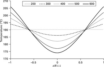
9.11 Influence of heater temperature on the yarn temperature profile. (adapted from Meier, 1993)
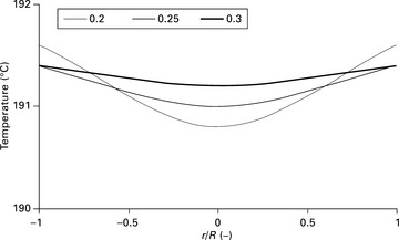
As Fig. 9.12 shows, the temperature of the core and the surface of the yarn can differ considerably at the beginning of the heater but are gradually equalized. In this example, the heater temperature was set to 200 °C and the fineness of the PET yarn was 167 dtex. Simulation results and measured values coincide very well as Fig. 9.13 shows. The slight deviations are due to a decreasing heat transfer coefficient with higher texturing speed in the practical trials whereas for the simulation a constant value was assumed.

9.12 Temperature of core and surface of the yarn over time. (adapted from Meier, 1993)

9.13 Comparison of calculated and measured values. (adapted from Meier, 1993)
9.3 Simulating fabric production: weft insertion and warp tension
In this section, the focus is on fabric production through weaving as the number of published papers on knitting and warp-knitting machines in English is relatively small.
9.3.1 Weft insertion
Lehnert (1994) developed a simulation tool in order to increase the number of picks in modern weaving machines. The most important factor limiting the machine speed was determined to be the number of yarn breaks due to tension peaks. In a first step, Lehnert thus analysed the yarn tension during weft insertion (Fig. 9.14). It is apparent that the tension increases at the beginning due to accelerating forces and is nearly constant when the yarn passes through the shed. Then at a machine angle of approximately 240°, a tension peak occurs which is due to the strong deceleration of the weft when the yarn is stopped by the yarn tensioner. The aim of the simulation model was to model the behaviour of the yarn under different conditions during the weft insertion and thus design a yarn tensioner that would be able to reduce this peak by applying a constant braking force. Based on a model devised by Wulfhorst (1969), Lehnert develops a model for the stress–strain behaviour of yarns during weft insertion. Figure 9.15 shows typical shapes of stress–strain curves for yarns. The curves show areas of elastic and of plastic deformation.
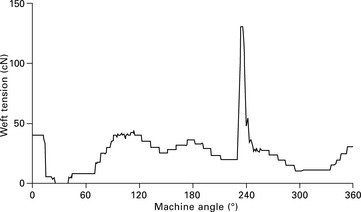
9.14 Weft yarn tension during weft insertion. (adapted from Lehnert, 1994)
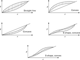
9.15 Typical shapes of stress–strain curves. (adapted from Hättenschwiler et al., 1984)
The elastic deformation at the beginning of the stress–strain curve can be described by
with c representing the spring constant and ε as the elastic elongation. In many cases, yarns become stronger with increasing strain, which can be described by

with Vstr = additional force due to the yarn strain.
If the stress–strain curve deviates from a purely elastic behaviour, we also have plastic deformation according to

Hence we get for the dependence between stress and strain
It is possible to describe all curves as shown in Fig. 9.15 with this equation, provided that the deformation velocity is infinitely small.
In reality, with deformation velocities as they occur during weft insertion, the force due to plastic deformation increases the more plastic the yarn is stretched. Then we have
with V = elongation parameter, ![]() = velocity of viscoelastic deformation and
= velocity of viscoelastic deformation and ![]() = initial value of the time-dependent additional force.
= initial value of the time-dependent additional force.
Hence we get for the force exerted on the weft during insertion
This mathematical model is depicted in Fig. 9.16. The parameters in equations [9.27] to [9.33] were determined experimentally until the resulting stress–strain curves coincided sufficiently well with the actually measured curves for different materials (e.g. PET filament yarn, PET OE-rotor yarn).

9.16 Signal flow chart of the yarn stress–strain model. (adapted from Lehnert, 1994)
The forces on the yarn during weft insertion are caused by frictional forces and forces of inertia. The latter depend on the yarn acceleration, its stress–strain behaviour and its mass. The forces of inertia can be calculated for a mass element representing the weft mass. This element exerts its force on the yarn at the end of the weft which is then considered without mass. Hence we have
Dividing the forces of inertia by the yarn mass, we get the weft acceleration. Integrating this equation twice, we get the distance which the weft has travelled for any given point in time during its insertion into the shed. This in turn affects the forces on the yarn according to its stress–strain behaviour and so forth. The respective signal flow chart is shown in Fig. 9.17.

9.17 Signal flow chart of the simulation. (adapted from Lehnert, 1994)
Figure 9.18 shows that simulation and actually measured yarn tensions coincide very well. As is shown in Fig. 9.19, with this model it is possible to determine the tension components which exert an influence on the weft yarn. It is apparent that the plastic deformation increases throughout the weft insertion. At the end of the weft insertion, two scenarios can occur.

9.18 Calculated and actual tension values during weft tension. (adapted from Lehnert, 1994)

9.19 Deformation of the weft yarn during insertion. (adapted from Lehnert, 1994)
• Firstly, the braking force of the tensioner on the yarn is too low, thus resulting in a yarn loop and a possible fault in the fabric.
• Secondly, the braking force of the tensioner on the yarn is too high, thus causing unnecessary plastic deformation and hence possibly a yarn break.
In order to avoid both, it would be helpful to have the braking force exerted by the tensioner on the weft at as low a value as possible. The simulation model developed here can be used to achieve this by simulating the forces exerted on the weft yarn during insertion which allows the optimum braking force of the tensioner to be calculated at any given time. As can be seen in Fig. 9.20, the simulation model does indeed optimize the weft tension considerably.

9.20 Comparison between yarn tension during weft insertion with and without a controlled yarn brake. (adapted from Lehnert, 1994)
A more recent model was published by Celik et al. (2004). It is based on the following equation:
where Fm is the force on the yarn from the main jet, FRJ,n are the forces of the relay jets, FSt stands for the force from the stretching nozzle, FB is the force of mass of inertia of the yarn from weft accumulator to the beginning of the reed, Fx represents the force of mass of inertia of the yarn through the reed, FA is the force applied to the yarn to unwind it from the bobbin and FR is the frictional force between yarn, machine components and air. According to their model, these forces are given by

with CR = yarn force coefficient according to de Jager (1990), Lm = length of the main jet and Pm = main jet air pressure,
with Cf = yarn force coefficient of the relay jets according to de Jager (1990), Vair = average air speed from the relay jets and Vy = weft speed. The yarn force coefficient was determined by measuring the force on the weft in the channel caused by the relay jets as a function of the air pressure.
The force by the stretching nozzle is regarded as constant:
The force of inertia on the yarn is given by
The force needed to unwind it from the bobbin is given by
The frictional force Fr can be expressed by
with f (t) = (1 − e[(t−Tsm)]/τ) for Tsm ≤ t ≤ Tem and f (t) = e(t−Tem)/2τ for Tem ≤ t, where Cfd stands for the frictional drag force coefficient for the weft, t is the running time, τ represents the pressure build-up time, Tsm the blowing start time and Tem the blowing stop time of the main jet. These equations lead to a nonlinear differential equation of the second order:
where x(t) stands for the position of the yarn tip while it travels through the reed and L2 is the distance between weft accumulator and beginning of the reed.
For the simulation, the initial values of weft position, velocity and acceleration are set to zero. Figure 9.21 shows a comparison of the calculated and experimental values for the weft speed for an OE rotor spun yarn. It is apparent that model and reality coincide well. This simulation method can be used to calculate and hence optimize, for example, the air consumption during weft insertion without having to resort to time-consuming trials.

9.21 Comparison between simulation results and measured values. (adapted from Celik et al., 2004)
9.3.2 Warp tension
In order to improve the machine settings without having to run expensive and time-consuming trials every time a new product is to be manufactured, a mathematical model describing the warp tensions was designed by de Weldige (1996). It describes the equilibrium of moments at the back rest of a weaving machine. The system and its boundaries are shown in Fig. 9.22. The boundaries are given by the point where the warp threads leave the warp beam and by the fabric beam. All weaving machine components that are taken into account are located above the grey plane.

9.22 System boundaries for the mathematical model. (adapted from de Weldige, 1996)
The equilibrium of moments at the backrest is determined by taking into account:
• the forces of mass inertia (1 in Fig. 9.22);
The warp tension is affected by the shed geometry, the weft beating up force, the fabric pattern and the weft density. The shed geometry and the weft beating up force are given by the machine parameters (3), fabric pattern and weft density result from the fabric parameters (4). Solving the equilibrium of moments leads to the movement over time of the backrest which in turn affects the warp tension. The control circuit is hence interconnected.
• The characteristics of all warp yarns are considered to be equal across the fabric width.
• Backrest, warp stop motion, sheds and reed are considered to be ideally stiff.
• The mass of the backrest is reduced to an equivalent mass; the springs and dampeners of the backrest are regarded as massless; their respective masses are taken into account in the equivalent mass of the backrest.
• The warp threads are considered to be spring elements with a linear stress–strain behaviour; this is allowed as the maximum elongation of the warp threads does not exceed 5%, which is well below the critical value of 10% where this assumption can no longer be made, as experiments show.
• The warp threads cannot take up pressure forces and are hence regarded as limp spring elements.
• The mass of the warp threads is several magnitudes smaller than the backrest mass and therefore neglected.
• The movement of heald frame and warp threads is the same, thus neglecting the heald allowance.
• The warp forces do not affect the movement of the heald frames.
• The influence of the warp stop motion drop wires on the warp threads is neglected.
• The frictional forces between thread guiding elements and the warp threads are not considered.
The warp forces are caused by the extension of the warp threads. Their absolute values for each heald frame depend on the geometric setting of the thread guiding elements, the shed geometry and the dynamic behaviour of all moving machine parts.
For a typical load situation, the stiffness of the warp threads is given by
The resulting warp force is hence
The overall tension Fges,i of the warp in heald frame i with m different warp yarns with j threads each and an elongation of εges,i is then given by
which leads to the overall warp tension
The model and all relevant parameters are shown in Fig. 9.23. This model is valid for Dornier and Picanol weaving machines, for example. All values are measured relative to a Cartesian coordinate system (X, Y) which originates at the tip of the front shed. This point was chosen since it does not move during the weaving process relative to the machine frame. In order to formulate the equilibrium of moments at the backrest, a relative coordinate system (X', Y') is used. For the conversion of one coordinate system into the other, we have

9.23 Schematic model of a weaving machine. (adapted from de Weldige, 1996)
The position of the backrest with unstretched warp threads can be described by the angle φ0. Its value can be calculated from the equilibrium of moments between the moment of equivalent mass of the backrest and the backrest spring forces. The latter can be determined using the overall spring constant cfsb and the spring length lfsbo. Hence, we have

The coordinate ![]() depends on the fabric pattern and on the machine angle, hence we have
depends on the fabric pattern and on the machine angle, hence we have
![]() can then be calculated according to
can then be calculated according to
assuming that heald frame i is in the upper or lower shed during the rest stage or does not move at all. Hence

with φstill = duration of heald frame resting stage in the open shed position [rad] and cbindung = indicator for the direction of the heald frame movement (+ 1: heald frame moves from upper to lower shed; –1: heald frame moves from lower to upper shed).
The thread length lkf,kbab is released by the warp beam according to
where ika stands for the overall gear ratio of the warp beam drive and φkb represents the absolute angle of the warp beam drive [rad] since the machine start (t = 0).
It can be determined for a PI controller according to

with φkb,tensioning = angle by which the warp beam was turned in a negative sense at machine start in order to achieve the given warp tension,
![]() φ(t) = controller deviation with
φ(t) = controller deviation with ![]() φ(t) = φ(t) – φsoll
φ(t) = φ(t) – φsoll
φsoll = given value of backrest position,
Tstart = starting point of warp let-off motion,
Kp(t) = proportional controller amplification with Kp(t) = Kp1 for t < Tkp;
Tkp = point in time at which the proportional controller amplification is switched from Kp1 to Kp2
Ki = integrating controller amplification,
Tski = point in time at which the integrating controller amplification is activated
nstart = rpm for warp let-off at machine start.
The warp load due to fabric take-up and reed beat-up is given by
The fabric take-up can be calculated with
where nwm stands for the number of picks per minute and densityweft represents the warp thread length per pick.
For the weft beating up, a sinusoidal warp thread extension according
Areed = amplitude of the fabric movement owing to the weft beating up
αreed-start = machine angle at which the fabric movement owing to the weft beating up commences
αreed-duration = duration of this fabric movement.
The elongation of each group of warp threads assigned to a certain heald frame can then be calculated with
The warp thread length lkfi(t) can be determined as the sum of the lengths of all warp thread segments between all components:
lkf, kb-sb = warp thread length between warp beam and backrest
lkf,sb = warp thread length across backrest
lkf, sb-kw = warp thread length between backrest and warp stop motion
lkfi,kw-s = warp thread length between warp stop motion and heald frame
lkfi,s-wr = warp thread length between heald frame i and fabric
lkf,kbab = shortening or lengthening of warp thread due to warp let-off motion
lkf,wrab = lengthening of warp thread by the fabric take-up
lkf,reed = lengthening of warp thread due to weft beating up.
The starting point of the simulation of the warp thread tension is given by
which is equivalent to the overall warp tension Fges reaching the given warp tension Fkf,soll.

Fges,x’ = Fges · [− cos (βl + β2) + sin (β3)]
Fges,y’ = Fges · [− sin (βl + β2) + cos (β3)]
lfsb = lfsbo for (lfsb–lfsbo) < 0
The movement of the heald frames and the weft beating up leads to a high frequency excitation of the system. Hence, the forces of mass inertia and dampening can no longer be neglected.
The law of the angular momentum at the backrest pivotal point is then given by
Apart from the constant parameters of the fabric and the machine, the solution of this equation depends on
• the time t since machine start;
• the angular velocity φ = dφ/dt;
• the ∫t ![]() φdt, which represents the integral of the deviation between backrest angle φ and given angle φreference.
φdt, which represents the integral of the deviation between backrest angle φ and given angle φreference.
The warp tension over time can then be calculated. The result for a typical example is shown in Fig. 9.24. The simulation of the warp tension makes it possible to determine an optimized machine setting (e.g. machine geometry) for any fabric prior to the actual trial thus saving time and hence money. This mathematical model was combined with evolutionary algorithms (see Chapter 3) to create the automatic weaving machine controller 'AUTOWARP' as described in de Weldige et al. (1997).

9.24 Comparison between measured and calculated warp tension. (adapted from de Weldige, 1996)
A similar approach to this concept was published in Grossmann et al. (2010). They describe a concept of a new weaving and take-up technology to produce complete spacer fabrics without a separate assembly process. In the last part, a mathematical model for the simulation of the dynamic warp thread forces was developed. It was used to dimension the roller drives and to avoid unnecessarily high warp thread forces and thus fibre damage. The basic equations are similar to those derived by de Weldige (1996). The warp threads are regarded as spring-damper elements, the machine elements themselves as nodes with mass and hence a resulting inertia force. Velocity and displacements are calculated using MATLAB©. A schematic block diagram of the model is shown in Fig. 9.25. Predicted and measured values of the warp tension show a good correlation. The model can hence be used to predict and thus also to minimize the warp thread tension in order to reduce yarn damage.
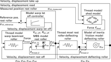
9.25 Block diagram of the simulation model. (adapted from Grossmann et al., 2010)
Kuo et al. (2010) present a model for the dynamic behaviour and the control of a horizontal cross-lapper. Their analytical approach is an excellent example of a thorough analysis of such systems and could also help other researchers designing models for other applications.
9.4 Simulating finishing techniques: rolling and dyeing
An elaborate model for an improved roller system with regard to bending rigidity was developed by Kuo and Vu (2011). They developed a new model for a roller made of steel and nylon by applying beam theory according to Timoshenko. The results of the simulation indicate that the new roller has a high dynamic response performance and is easier to keep in a stable state than conventional rollers. A comparison between calculated and actually measured values for the new system is yet to be published. Other papers on the simulation of controllers for calendar roller systems worth reading include Kuo et al. (2011a, 2011b).
A mathematical description of a complete package or packed bed dyeing machine was published in Burley et al. (1985). The processes of convection, dispersion, absorption and desorption of dye to and from the packed bed of fibres were modelled, while account was also taken of the addition of dye to, and the possible removal of liquor from, the mixing tank. A numerical simulation of the mathematical model based on finite differences was developed and numerical results presented. Techniques for monitoring the accuracy of the results based on conservation properties of the system were discussed. Formulae for the expected theoretical steady states of the system were also given.
9.5 Simulating plant layout and production planning: finishing operations
Plant design and production planning are important issues in order to run a textile mill successfully. The main objective is to optimize the process flow by reducing queuing time, thus increasing the output of the plant. At the same time, the waiting time for customers to receive their ordered goods can also be decreased which is an often neglected but nevertheless important factor for the success of a textile enterprise.
An early noteworthy paper that deals with the optimized design of a textile mill is Livingston and Sommerfeld (1989). They apply the general purpose simulation system (GPSS) to perform a discrete-event simulation of a textile finishing mill that produces a variety of dyed and finished woven and knit fabrics. The GPSS is based on the queueing theory where the queue represents in this example work-in-process (WIP) inventory, batch chemicals or a custom order. The results of the simulation are, for example, machine utilization, queue length, WIP and idle time, production and residence time of one unit in the overall model. They can be used to calculate operator availability, possible bottlenecks, storage requirements and also to simulate stochastic behaviour of the operators, customers and the process itself. The aim of the simulation was to determine, among others, the impact of market demands, maintenance practices, quality control policies, capacity increase on equipment and manpower utilization, total production and manufacturing time on the overall performance of the mill. The flow diagram of the mill that was analysed is given in Fig. 9.26.
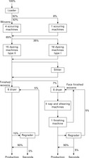
9.26 Flow diagram of textile finishing mill. (adapted from Livingston and Sommerfeld, 1989)
After the loader unloads the wovens (92% of total production), they are cleaned in one of four scouring machines, the knits (8%) are cleaned in the fifth. All fabrics are then dyed in one of 33 dyeing machines. Some 15% of the wovens are checked after inspection by a regrader. Normally, 90% pass this test, 5% are sent back to the dryers and 5% are marked as seconds. In contrast, the knits are sent from the dyeing machines to the slitter, dried, napped, sheared and inspected. Again, 15% are checked by a regrader similar to the wovens. Besides this production process, also preventive maintenance procedures were taken into account.
The model is divided into segments which contain, for example, the machines and the queues before the machines. Figure 9.27 shows a typical example for the loading and scouring process: the loader distributes the fabrics to the knit scouring machine (8%) and the wovens scouring machines (92%). There, they are processed which is represented by queue-enter-depart-advance-leave operations. Each is assigned a certain time and capacity which can then be changed in the model. In a similar way, maintenance intervals are incorporated.

9.27 Model segment for loader and scouring machines. (adapted from Livingston and Sommerfeld, 1989)
The authors then changed several parameters to determine their effect on the overall performance of the mill which led to the following results: an increase of the percentage of knits from 8% to 20% led to an increase of the one scouring machine utilization from 22% to 50% with no significant change in any of the other output results. Similarly, changes of other parameters such as the percentage of face-finished goods from 7% to 15%, the number of regraders and the percentage of re-inspected goods did not greatly affect the overall performance of the mill. In contrast, when the loader time was decreased which is equivalent to an overall production increase, it became apparent that the dyers were a bottleneck. A production increase by 17% could be managed with just one additional dyer whereas an increase by 33% required five additional dye machines to be added as can be seen in Fig. 9.28.

9.28 Production parameters change for a 33% decrease of loader time. (data taken from Livingston and Sommerfeld, 1989)
A recent paper by Azadeh et al. (2010) describes a more elaborate approach for a finishing mill which includes goal programming and a design of experiment (DoE) algorithm to optimize a mill with not just one but multiple objectives. It also gives references to a number of papers about the general approach of production planning. A schematic overview of the production process which was analysed is depicted in Fig. 9.29. Six different goods are produces using between one and three processes.

9.29 Schematic overview of the production process. (adapted from Azadeh et al., 2010)
The main objectives were to minimize the completion time of each process, thus ensuring on-time delivery of the goods, and to decrease the processing times of all machines, hence lowering machine depreciation and other related costs. Typical assumptions such as 'all jobs are available at the starting time of the scheduling problem', 'one job cannot be allocated to more than one machine at the same time' and 'the processing time of each job on each machine includes setup times, transportation time', etc. were made.
With regard to the main objectives, the following five decision parameters were considered:
• specification of dyeing machines;
• working with either existing low technology machines or replacing them with high technology ones;
• temperatures of the printing and the stenter machine;
• the number of stenter machines; and
• five different workshop dispatching rules (e.g. first in first out, last in first out).
A different number of levels was assigned to each of the four factors which would have resulted in too large a number of possible combinations to be calculated. Hence, a complete factorial design using only the maximum and minimum values was employed which reduced the number of combinations to 5 × 24 = 80. By carrying out an analysis of variance (ANOVA), parameters which have no significant impact on the result are eliminated.
The simulation led to the following conclusions: set temperatures of printing and stenter machine to certain values, double the number of stenter machines, continue working with two low technology dyeing machines, the best dispatching rule is 'first in first out' and three extra workers are needed. This approach could also be applied to other kinds of textile mills and seems to be very promising with regard to an easy-to-use system for the optimization of plant design and production planning.
9.6 Practical advice in simulating textile machinery
Before trying to create an accurate model of reality, it is advisable to define the goal which is to be achieved by the simulation. This in turn requires a thorough analysis of the relevant parameters as an important and indispensable step. From there, designing a simplified model which still represents the real case with sufficient accuracy is the next step. In many cases, it is fully sufficient to consider not the machine as a whole but only certain crucial components which may separately be modelled much more easily than the entire system. In some cases, where one model does not fit reality, it is a sensible approach to create separate models for a certain parameter range. This often simplifies the simulation.
Whereas in the 1980s and 1990s most simulation programs were written by researchers from scratch, today there is a wide range of commercial tools available with which even complex models can be created. Engineers striving to describe textile machines and processes should hence concentrate on tailoring these programs to the problem in question rather than doing all the programming themselves.
Without the means to verify the results, a simulation of machines or components is pointless. Nevertheless, many papers that have been published in recent years do not present means to actually compare the calculated results with measurable values. Hence, a large number of papers describing such models have not been considered in this chapter although the simulation results appeared to be sensible.
9.7 References and further reading
Azadeh, A., Ghaderi, S.F., Dehghanbaghi, M., Dabbaghi, A. Integration of simulation, design of experiment and goal programming for minimization of makespan and tardiness. International Journal of Advanced Manufacturing Technology. 2010; 46:431–444.
Basligil, H. Determining machine interference through simulation method and its application to textile industry', Modelling, Measurement & ControlD: Manufacturing, Management. Human & Socio-Economic Problems. 1994; 9(1–3):23–42.
Batra, S.K., Ghosh, T.K., Zeidman, M.I. An integrated approach to dynamic analysis of the ring spinning process. Part I: without air drag and Coriolis acceleration. Textile Research Journal. 1989; 59(6):309–317.
Batra, S.K., Ghosh, T.K., Zeidman, M.I. An integrated approach to dynamic analysis of the ring spinning process. Part II: with air drag. Textile Research Journal. 1989; 59(7):416–424.
Baykara, M., Öznergiz, E., Özsoy, C., Demir, A., Gülsen, S. The air-jet texturing and twisting machine's and model predictive control based on state-space', Proceedings of 2nd IFAC International Conference on Intelligent Control Systems and Signal Processing, vol. 2. Part. 2009; 1:73–78.
Braccesi, C., Carfagni, M. Using simulation to optimise output from an open-end rotor-spinning machine. Journal of the Textile Institute. 1993; 84:107–119.
Burley, R., Wai, P.-C., McGuire, G.R. Numerical simulation of an axial flow package dyeing machine. Applied Mathematical Modelling. 1985; 9(1):33–39.
Celik, N., Babaarslan, O., Bandara, M.P.U. A mathematical model for numerical simulation of weft insertion on an air-jet weaving machine. Textile Research Journal. 2004; 74:236–240.
Crank, J. A theoretical investigation of cap and ring spinning systems. Textile Research Journal. 1953; 23:266–276.
Crank, J., Whitmore, D.D. Balloon diameters and thread tensions calculated for different cap-spinning conditions. Textile Research Journal. 1953; 23:657–663.
Crank, J., Whitmore, D.D. The effect of cap-edge friction on spinning. Textile Research Journal. 1954; 24:434–437.
De Jager, G. Untersuchung und Simulation des Schusseintrags an Luftdüsenwebmaschinen. Mitt. Inst. Textilmasch. Textilind. (25):1990.
De Weldige, E. Prozeßsimulation der Kettfadenzugkräfte in Webmaschinen', doctoral thesis. RWTH Aachen University; 1996.
De Weldige, E., Osthus, T., Wulfhorst, B. Reducing set-up times and optimizing processes by the automation of setting procedures on looms. Mechatronics. 1995; 5:147–163.
De Weldige, E., Osthus, T., Wulfhorst, B. Auto-warp process optimization and increased production through fully automatic loom setting. Melliand Textilberichte. 1997; 78:141–143.
Greenwood, K., Grigg, P.J. The development of twist in a false-twist texturing machine with a friction twister. Journal of the Textile Institute. 1985; 76:244–263.
Grossmann, K., Muehl, A., Loeser, M., Cherif, C., Hoffmann, G., Torun, A.R. New solutions for the manufacturing of spacer preforms for thermoplastic textile-reinforced lightweight structures. Production Engineering Research Development. 2010; 4:589–597.
Hättenschwiler, P., Pfeiffer, R., Schaufelberger, J. Die Zugfestigkeit von Garnen (Neue Erkenntnisse aus der Praxis). Melliand Textilberichte. 1984; 65(23–26):98–107.
Kuo, C.-F.J., Vu, H.Q. Dynamic modeling and control of a bending combined roller system using Timoshenko beam theory and constrained model predictive control. Textile Research Journal. 2011; 81:1448–1459.
Kuo, C.-F.J., Tu, H.-M., Liu, C.-H. Dynamic modeling and control of a current new horizontal type cross-lapper machine. Textile Research Journal. 2010; 80:2016–2027.
Kuo, C.-F.J., Chen, J.-S., Hiep, P.V., Tu, H.-M. Theoretical control and experimental verification of a calendar roller system, Part 1: dynamic system modeling and model predictive controller design. Textile Research Journal. 2011; 81:10–21.
Kuo, C.-F.J., Chen, J.-S., Hiep, P.V., Tu, H.-M. An entire strategy for control of a calendar roller system, part 2: settling time-optimal feedback control. Textile Research Journal. 2011; 81:542–549.
Lehnert, F., Simulation und Reduzierung der Schußfadenbelastung beim Webendoctoral thesis. RWTH Aachen University, 1994.
Livingston, D.L., Sommerfeld, J.T. Discrete-event simulation in the design of textile finishing processes. Textile Research Journal. 1989; 59:589–596.
Meier, K., Shortening of the heating zone in false-twist texturing. Proceedings of 32nd International Man-made Fiber Conference. Dornbirn, 1993:1–8.
Olbrich, A. Analyse und Simulation der Drallerteilung durch Friktion zur Optimierung der Falschdraht-Texturierung', doctoral thesis. RWTH Aachen University; 1995.
Osterloh, M., Wulfhorst, B. Opportunities for energy saving in the texturing process. Chemical Fibers International. 1996; 46:364–366.
Tang, H.B., Xu, B.G., Tao, X.M., Feng, J. Mathematical modelling and numerical simulation of yarn behaviour in a modified ring spinning system. Applied Mathematical Modelling. 2010; 35:139–151.
Tang, H.B., Xu, B.G., Tao, X.M. A new analytical solution of the twist wave propagation equation with its application in a modified ring spinning system. Textile Research Journal. 2010; 80(7):636–641.
Wulfhorst, B. Formänderungseigenschaften von Polyurethan- und KautschukElastomerfäden', doctoral thesis. RWTH Aachen University; 1969.
Zhu, M., Wang, Z. Textile spinning-frame roller fault diagnosis based on improved wavelet analysis and support vector machine. Proceedings of International Conference on Electric Information and Control Engineering. 2011; 786–790. [2011].