Computational fluid dynamics (CFD) and its application to textile technology
Abstract:
Computational fluid dynamics (CFD) deals with numerical flow simulation. By applying CFD, even complex problems can be solved using a numerical iteration process. A commonly used method involves the Navier–Stokes equations which represent a system of equations for continuity, impulse and energy conservation of a fluid. Typical examples for the simulation of complex flows are the air current around aircrafts and inside cars, and the modelling of heat transfer for a wide range of applications, including in textile processing.
5.1 Introduction
All programs that simulate currents are based on equations describing fluid mechanics. Those date back to Roman times when canals, baths and aqueducts were built using laws of fluid mechanics. Leonardo da Vinci (1452–1519) used fluid mechanics for various applications, e.g. to describe water passing obstacles. Important contributions were made between the seventeenth and the nineteenth centuries by Isaac Newton (1643–1727) with the three axioms of classic mechanics, by Jakob I. Bernoulli (1655–1705) with the one-dimensional energy equation and by Leonhard Euler (1707–1783) who described the law of impulse conservation for frictionless currents.
Two of the most important researchers in the field of fluid mechanics were Claude Navier (1785–1836) and George G. Stokes (1819–1903). Their findings allowed the extension of Euler's equation using the Navier–Stokes equations by taking into account the influence of friction. Although originally regarded as of not much use, today the Navier–Stokes equations are the basis for most computational fluid dynamics (CFD) software. Because of its complexity, CFD can only be solved using an iterative, numerical approximation, which still requires a powerful computer. Calculation time varies, depending on the problem at hand, between fractions of seconds and months.
More recent contributions include Rodi and Spalding (1970) who implemented several algorithms that are still used today. Another important contribution was made by Baliga and Patankar (1980). The first commercial CFD software became available in the 1980s. It was firstly used by the aircraft industries. Since the 1990s, CFD simulations have been widely used, e.g. in the automotive and the textile industries. Today, CFD is an accepted part of computer-aided engineering (CAE). Good introductions into CFD and the theory behind it can be found in Abbot and Basco (1989), Bhaskaran and Collins (2008), Cebeci et al. (2005), Hirsch (2007) and Mason (1998).
5.2 From reality to simulation
Today, a wide range of commercial CFD software is available (see Section 5.9). Nevertheless, it is of crucial importance that the user is familiar with simulation in general and also with the physical laws that apply in order to select a suitable model and the respective algorithms. This is a major difference to many other simulation tools (e.g. neural networks). This is illustrated in Fig. 5.1.

Starting from reality, the first step includes abstracting and creating a model which should be kept as simple as possible. This already incorporates the possibility of an error which should not be underestimated. A thorough analysis of the laws governing the problem and hence a suitable model is crucial for the success of the simulation. In subsequent steps, applying the model first leads to the physical relations between the parameters, then a numerical representation, subsequently to the actual simulation and final results which are to be verified. During each step, the user is advised to check for errors so as not to distort reality beyond acceptable limits or to achieve a completely wrong solution.
Common sources of error of a CFD simulation are:
• simplification of reality, hence not all aspects and details are taken into account;
• inaccuracies of the solution due to rounding errors depending on the numerical algorithms which are used;
As Fig. 5.2 shows, choosing a suitable number of nodes to represent the current flow profile is a decisive step. In this example, the parabolic velocity profile can be approximated by three nodes with a trapezoidal cross-section which represents an easy-to-calculate solution. However, using 15 nodes leads to a solution which coincides much better with the original parabolic profile. In the end, every simulation solution is only as good as its validation which is thus an indispensable part of the process. It must be noted though that it is very difficult to measure currents without affecting the current itself and also that measuring inaccuracies are not uncommon.
5.2.1 Reality
Most phenomena involving the flow of a fluid are very complex in reality. In order to describe them, a certain degree of abstraction is necessary which still takes into account all relevant parameters and conditions. For example, one milligram of water consists of approximately 3.3 × 10¹⁹ molecules with different velocities. It is impossible to create a model which incorporates each molecule separately. Hence, water is normally regarded as a continuum having a constant density and temperature if only the macroscopic, integral forces are of interest.
5.2.2 Model
As described above, a model normally only describes the influence of those parameters that are considered to be of importance. If non-relevant parameters are not taken into account, the model becomes more complex without improving the final results. If, in contrast, relevant parameters are neglected, the model will often not mirror reality to the desired extent. Typical examples of models for a CFD simulation are:
• Water waves: in order to design a model that simulates wave propagation, water is regarded as a continuum. Friction effects in the water and between water and air are neglected. Also temperature, water colour and the number of living beings within the observed volume are not relevant. Salt content is represented by the average density. Important parameters include the distance between wave crests (wave length), wave amplitude and gravitational force.
• Perfusion of fabrics: a fabric made up of staple fibre yarns represents a very complex geometrical problem for a flow simulation. It consists of a large number of intersecting yarns which in turn are built up of single fibres. For an outdoor application where the fabric is subjected to wind, an intimate knowledge of the current around each single fibre is not relevant. Hence, applying an air resistance factor of the fabric relative to the air velocity would be sufficient to model the fabric as a flat area.
• Polymer flow in melt spinning: melt distribution inside a spin pack can be simulated by regarding the temperature as isothermal despite its high value. However, density and viscosity of the melt must be adapted to the spin temperature.
In order to create a model for fluids, there is a wide range of possibilities, namely:
• Lagrange approach: a fluid particle's (molecule, atom, agglomerate) trajectory is observed and its properties are recorded. As a result, the time-dependency of the parameters is recorded but not their dependency on a position. A typical example are currents of granulate or sand.
• Euler approach: the flow field is regarded as a continuum which allows to determine the parameters depending on their location.
• Euler-Lagrange approach: this is a combination of both approaches and is especially suitable for the description of single particles in a continuous medium, e.g. the movement of fibres or yarns in a current.
To illustrate these approaches, one can make a thought experiment: if a continuous flow is recorded for a given point in time, this results in a description according to Euler. If a fluid particle in this field is marked repeatedly at given time intervals, this results in a series of Euler fields. By connecting the marked particle hence obtaining their trajectory, one obtains a description according to Lagrange.
5.2.3 Physical relations
After determining the parameters of the model by abstracting reality, they need to be connected applying the laws of physics. Newton fluids, e.g. air and water, can be described according to Euler's approach using the Navier–Stokes equations, provided that the laws of continuum mechanics apply. They make up the all-embracing model for the description of fluids, and consist of a system of non-linear, partial differential equations of the second order which describe a continuous flow, taking into account friction and heat conduction.
The conservation equation for mass is given by:
According to equation [5.1], the sum of time-dependent change of the density ρ and the three-dimensional change of the current density ![]() is nil. The mass of the current is preserved.
is nil. The mass of the current is preserved.
The conservation equation for impulse is given by:
The term ![]() represents the dyadic product of the velocity, with
represents the dyadic product of the velocity, with
which, when multiplied with the density, results in ![]() . The term
. The term ![]() stands for the tension tensor. The areal change of the sum of impulse flow and tension, added by the time-dependent change of the flow density, results in the volume force.
stands for the tension tensor. The areal change of the sum of impulse flow and tension, added by the time-dependent change of the flow density, results in the volume force. ![]() which can be equal to, for example, the gravitational force, hence we have
which can be equal to, for example, the gravitational force, hence we have ![]()
The conservation equation for energy is given by:
The time-dependent change of the energy per volume unit ρE, added by the areal change of the sum of the energy flow ![]() , the power of the tensions
, the power of the tensions ![]() and the heat flow
and the heat flow ![]() is equal to the power of the volume forces
is equal to the power of the volume forces ![]() The conservation equations for mass, impulse and energy also include deduction after time. These can be neglected for stationary processes so that only the stationary conservation equations remain.
The conservation equations for mass, impulse and energy also include deduction after time. These can be neglected for stationary processes so that only the stationary conservation equations remain.
5.2.4 Numerics
Numerics are a subarea of classic mathematics. The respective approaches are mainly used to solve equations, in most cases with a computer. Some physical relations can be determined analytically. Others, such as systems of partial equations, are normally solved numerically via an iteration process. The equations are then discretized into algebraic equations.
Discretization
By applying a time discretization, the process is analysed at different points in time. Similarly, a local discretization implies the division of the geometry into small parts which are then analysed separately. According to Lohner (2008), this results in either structured or unstructured cross-linkings, which can be defined as follows:
• micro-structured: each node within the net is surrounded by the same amount of adjacent nodes;
• micro-unstructured: each node within the net is surrounded by a different amount of adjacent nodes;
• macro-unstructured, micro-unstructured: each net consists of sub-meshes which are micro structured.
Figure 5.3 shows the cross-linking of a volume with a structured (left) and an unstructured (right) cross-linking.

The discretized equations are then linearized in order to transform them into a numerically solvable system of equations which represents the whole flow field. According to Peiró and Sherwin (2005), the most important methods of discretization are:
When using the finite differences method, the current is represented by single points. This comparatively simple method is especially suitable for structured grids and one-dimensional problems. This method can cause convergence problems for a steep gradient.
When using the finite volume method, the current is converted into basic functions with several degrees of freedom. Their programming is complex but this method allows the simulation of any unstructured grid. Steep gradients can be taken into account with special algorithms. The finite element method is a direct approximation of the integral conservation equations. It is common to solve problems related to flow simulations. Mass, impulse and energy are preserved. Owing to their integral form, the equations can be used for discontinuous problems as well as for unstructured grids. Figure 5.4 shows a comparison of the three methods.
![]()
5.4 Comparison between finite differences, finite element and finite volume method. (adapted from Roller et al., 2005)
The discretized systems of equations can be approximated using a range of approaches, all striving to achieve convergence via iterative approaches. In general, there are the following methods:
• One-step method: data about the solution curve are used for only one time step in the interval [tn-1, t1]. Hence, this method takes data into account only of point in time tn-1, but not those of previous steps. The timespan Δt determines the congruence behaviour of the solution. It is sufficient to set the starting point, hence the method is called 'self-starting'.
• Multi-step method: this method also uses data prior to tn-1, hence taking several steps into account. It is not suitable to numerically solve complex, dynamic systems as the determination of data sets prior to the current set is a time-consuming process.
• Explicit method: this method is the most simple time discretization process. The new values of the parameters at point in time tn+1 can directly be deducted from those at point in time t. Its main advantage is the easy and hence quick dissolution of the system of equations. Its drawback is the limitation of the increment due to numerical instability.
• Implicit method: this method does not have that restriction, but the time required to calculate the values for each time step is much greater. Hence, this method is preferred for applications with large increments, especially when convergence for a stationary flow is an issue.
Turbulence models
Turbulence in the current can have a direct effect on the flow field. It is often caused by surface irregularities or barriers blocking the current. Normally, the average flow velocity is superimposed by a time-dependent velocity oscillation. In contrast to a laminar flow, this can cause a mixing of the various flow layers. The current velocity of a turbulent flow is given by
where ![]() stands for the average velocity over time and
stands for the average velocity over time and ![]() represents the turbulence component of the velocity.
represents the turbulence component of the velocity.
A turbulent flow is characterized by the degree of turbulence Tu. It represents the size of the time-dependent oscillations of the flow velocity relative to the average velocity. For a three-dimensional flow field, it can be calculated as follows:
where u',v’ and w' stand for the oscillation components of the flow speed.
Figure 5.5 shows the time-dependent oscillations of a turbulent flow for high and low values of Tu. The time-dependent oscillations of a turbulent flow can be explained by vortex-like structures within the current. The so-called eddies are three-dimensional structures which can be as large as the current itself and as small as a single fluid particle. Whereas the large eddies cause an exchange of impulses within the current, the small eddies transform turbulent energy into heat through dissipation.
Several models are used to simulate a turbulent flow.
Reynolds-averaged Navier–Stokes equations (RANS)
The Reynolds-averaged Navier–Stokes equations (RANS) are most commonly used in engineering. They do not disintegrate turbulent structures with regard to time and location but model the relevant parameters through a turbulent kinetic energy approach. This is a comparatively quick method which normally leads to good results.
Standard k-ε turbulence model
This model was developed by Launder and Spalding (1974) and describes the development of the turbulent, kinetic energy k and the isotropic dissipation rate ε. It leads to viable results for those areas away from the surrounding wall. The isotropic dissipation rate ε represents the kinetic energy of the turbulent flow which is either transformed or dissipated into inner energy (heat) per time and mass unit. Energy is extracted from the main current by large turbulence elements and passed on to smaller elements.
K-ω turbulence model
Salari et al. (1994) developed another model which can also be used to describe the flow field close to the surrounding wall and in shear layers. It describes the relation between kinetic energy k and the speciic, isentrope dissipation rate ω according to:

where lt represents the eddies' length. This model is very sensitive to small changes of the turbulence parameters at the edges of the flow field.
Shear-stress transport k–ϖ model
The so-called shear-stress transport (SST) model was invented by Menter (1994). It combines the advantages of the aforementioned models, shows a higher accuracy and is more reliable while still requiring the same computing time. In areas close to the wall, turbulence is described applying the k-ω model, in areas away from the walls, the k-ε model is used. A transition function is defined which assumes values between 0 and 1. This value is multiplied with the respective function and both functions are then added. The distinguishing feature of this model is how the flow at the wall is simulated. If the node which is nearest to the wall is further away from it than a deined distance, the wall function of the k-ε model is used. If it is closer, then the Low-Reynolds equation (for currents with low Re numbers) is gradually taken into account. This meets on the one hand the general demand for a sufficiently high number of nodes in order to describe the flow with a high degree of accuracy. On the other hand, the automatic switch to the Low-Reynolds equation ensures that, independent of the grid resolution, the flow close to the wall is always described properly.
5.2.5 Simulation
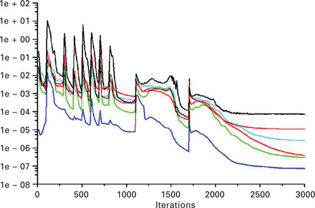
During the simulation, numerical methods are applied in order to solve the equations representing the governing laws of physics. In CFD, this is normally a finite element method and hence an iterative process. Thus, in the beginning, to each cell, a starting value for velocity, turbulence and pressure is allocated. This initial solution is then converted to the actual solution step-by-step. This convergence process can be supervised by determining the residues. They represent the difference between the current solution and the true solution. This can be achieved by observing the relevant parameters, e.g. maximum flow velocity or temperature at the outlet. If both convergence criteria are met, the simulation can be terminated as the flow field will not change any more.
If the initial solution is too far away from the true solution, the process can be divergent which requires ending the simulation. In this case, it can be useful to adjust the boundary conditions step-by-step to their final values. A typical example is a supersonic current where the simulation starts with a low pressure which is then gradually increased to the maximum value. Plate I (see colour section between pages 152 and 153) shows a typical example of the development over time of the residuals.
5.2.6 Validation
After the simulation, each cell is described by values that characterize the state of the cell within the current. From them, the necessary information to describe the flow must be extracted. One possibility is to export the numerical result as single values or in tables, another their summary in diagrams for velocity and pressure over time, yet another the three-dimensional depiction of the flow. The main difficulty is the presentation of the results in such a way that users receive the information they want.
A plausibility test is an indispensable part of every validation. This can simply be done by checking whether the current flows into the right direction and whether all boundary conditions are met. In addition, sophisticated measuring technology can be employed to validate the simulation in certain areas (see Section 5.4).
5.3 Simulation of currents with fibres, yarns and textiles
For many applications in textile technology, apart from the movement of the flow, the movement of fibres and yarns inside the flow is also of great interest. This leads to coupled simulations where fibres and yarns move freely through a current and are in turn affected by it. In most cases, the preferred model to tackle this problem is the inite volume method. Fibres and yarns are then not regarded as a continuum but as single objects and hence treated separately.
If ibres and yarns are to interact with the current, there must be an interface at which an exchange of impulse can take place. Fibres and yarns are normally longer than they are wide; typical ratios are in the range of 1000:1–100 000:1. Besides, the geometrical dimensions of the current are in most cases much greater than the fibre or yarn diameter. Magnitude differences between the smallest (ibre) and the largest (machine) dimension can reach 1 000 000 and more.
One possibility to exchange impulses between yarn and current is the body-fitted-mesh method (Fig. 5.6, top). There, the yarn is completely integrated into the grid that describes the current. This implies an enormously high number of nodes and the calculation step in each time interval is very time consuming. The great advantage of this method is though that the exchange of impulses can be directly determined via turbulence models as described above.

5.6 Different methods to model a fibre or yarn in a current (top: body-fitted mesh; middle: immersed-boundary-layer; bottom: unchanged net).
An alternative is the immersed-boundary-layer method as described by Lai and Peskin (2000). In a cartesian mesh, those nodes surrounding the fibre and the yarn are distributed until the desired mesh ineness is achieved. The other nodes are distributed evenly (Fig. 5.6, middle). The major advantage of this method is the considerably lower number of nodes required and hence a much shorter computing time. However, in order to represent the exchange of impulse for turbulent flows, separate models need to be defined.
A third possibility as shown in Fig. 5.6, bottom, is an unchanged net. This approach is similar to the immersed-boundary-layer method but the mesh is not denser close to the ibre or the yarn. This method can then be applied when ibres or yarns cover more than one cell which makes a reinement of the mesh to describe the different flow forces onto the fibre or the yarn dispensable.
When using the last two approaches, separate methods to describe the exchange of impulse must be deined by applying resistance factors. A good summary is published in Marheineke and Wegener (2009). A major challenge are fibres or yarns that flow against the current at angles smaller than 5°. Plate II shows the simulation result of a single, crimped fibre in an air flow and illustrates the complex conditions.

Besides the interactions of the fibre and the yarn with the fluid, interactions with walls and other ibres and yarns must also be taken into account. Another dificulty is the representation of elasticity in such a simulation. When considering this parameter, the time increment becomes very small as the computing algorithm otherwise becomes unstable. According to Courant et al. (1928), the maximum time increment can be calculated by
Equation [5.8] implies that the maximum time increment increases with density ρ and segment length Δl and decreases with the E-modulus of the fibre or the yarn.
5.4 Validation methods
Apart from the plausibility tests as described above, the validation of the simulation results by measuring the actual current is very important to assess the quality of the model and the results. In the following, three commonly used methods to measure the flow velocity are described briefly.
5.4.1 Laser Doppler anemometry (LDA)
Here, the inference pattern of two coherent laser beams is used to determine the speed of particles within a current. The laser beam is first separated by a beam divider. The two phase-delayed beams are then brought into focus using a lens so that an interference pattern made up of bright and dark spots arises as shown in Fig. 5.7. Tracer particles brought into the current move through this light pattern and start to light up in a velocity-dependent frequency. This frequency is detected and the respective value converted into a velocity. The main advantage of this method is that the current is not affected as this is a purely optical technique. The main disadvantage is the extraordinary high price for the necessary equipment which can easily reach € 250 000. An interesting paper on the subject was published by Lehmann (1988).

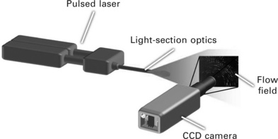
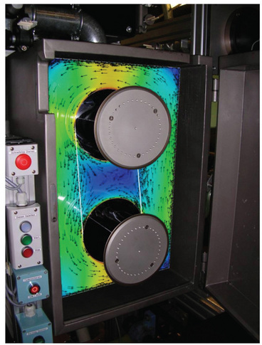
5.4.2 Particle image velocimetry (PIV)
The principle of Particle image velocimetry (PIV) is based on the time-dependent measurement of the position of particles (so-called seeds) moving through the current. One layer of the current is subjected to two very brief light impulses (duration in the range of nanoseconds) within microseconds. The displacement of the particles over time is recorded via CCD or CMOS camera for the points in time t and t’. Applying a cross-correlation, the particle distribution in this layer at t and t’ can then be detected. Normally, 10 000 velocity vectors can be calculated for one frame. By averaging up to several hundred measurements, a velocity chart can be drawn. Figure 5.8 shows the principle of PIV.
When using a second PIV system with another camera, it is possible to realize a stereo measurement. Hence, the velocity vectors can be determined in three dimensions. This principle is applicable for small and large volume flows and for a wide range of flow velocities ranging from a few mm/s up to 1 km/s. The main advantage of this method is that the result is a two dimensional vector field which mirrors the flow. This makes it easy to determine areas of turbulence and laminar flow which is very difficult with LDA measurements. A detailed explanation of the measuring principle can be found in Raffel et al. (2007).
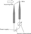
5.4.3 Hot-wire anemometry (HWA)
With this method, air flow velocities can be measured. The principle is based on the cooling effect of an air flow on a hot wire which depends directly on the flow velocity (Hussein, 1990). By keeping the hot wire at a constant temperature, a dissipation loss can be recorded which depends on the fluid velocity. Air temperature and humidity at the beginning of the measurement have a direct effect on the result. Hence, the hot-wire sensor must be calibrated before the actual start of the measurement. Figure 5.9 shows the principle of hot-wire anemometry (HWA). The main advantage of this method is its easy applicability in contrast to LDA and PIV for which the technical equipment is much more complicated. Another advantage is the possibility to record fluid velocity continuously at a frequency of several kHz. This allows the measurement of laminar and also turbulent flows.
Besides these three methods, there are other techniques, such as measuring
5.5 Economic aspects
The simulation of currents is one of the most expensive methods to optimize a process. The usage of the costly software requires a thorough knowledge in fluid dynamics, different modelling techniques and the algorithms used to solve the problem. This makes CFD simulations different from the methods described in Chapters 2–4 where even a little knowledge can lead to viable results. Hence, in many applications, prior to receiving the first usable results, high costs can arise from personnel and software. In some cases it is thus easier and cheaper to achieve results by using empirical methods or by simply measuring the currents. But for complex problems, CFD often is the only possible way to tackle them.
An empirical approach is the most simple and obvious method to optimize a process: based on existing knowledge and results of trials, dependencies between the interesting parameters are derived. If the number of influencing parameters is small and their relations are clear, an empirical approach often leads quickly to first results, thus allowing a process optimization at little cost.
By using measuring instruments, the influencing parameters can also be quantified so allowing conclusions to be drawn of the fundamental laws governing the process. Typical examples are temperature sensors or position measuring devices. The necessary instrumentation can become very complex depending on the problem to be solved (Ramakers, 2005; Ramakers et al., 2006). An important aspect when using measuring instruments is the determination of the measuring range and accuracy which in turn has a direct effect on the costs.
In many cases, an empirical approach in combination with measuring techniques is limited due to boundary conditions. Then, CFD is an interesting alternative although it requires a considerable amount of preparation: the geometrical conditions must be fed into the model, the boundary conditions must be defined and suitable models must be chosen in order to achieve usable results. Besides, it is of crucial importance with regard to costs and computing time to define the required accuracy of the model at a very early stage.
The major benefits of CFD modelling versus empiricism are hence:
• currents can be depicted in three dimensions and are time-dependent;
• details inside the current can be shown which could not be detected by pure measurement;
• geometries can be analysed that only exist in virtual reality;
• parameter values can be analysed within a wide range without the need to build expensive prototypes;
Empiricism, measuring technology and simulation are compared qualitatively in Fig. 5.10 by showing costs of process optimization versus process quality.
![]()
5.10 Costs of process optimization vs. process quality for empiricism, measuring technology and simulation.
By using empiricism, it is possible to achieve improvements with comparably small investment by changing parameters, e.g. of a machine, ever so slightly until a certain criterion is met. The curve in Fig. 5.10 shows a slow increase which levels out after some time. From this point on, it is very hard to further improve the process. The main reason for this is the missing understanding of the process and the interactions between the different parameters.
When using measuring technology to optimize a process, costs arise due to the initial investment. This leads with a delayed increase of the process quality compared with empiricism. The curve then increases quicker and reaches a higher level, owing to a better understanding of the process itself. At a certain point, the curve levels out as not all interactions between the process parameters can be determined.
For a typical CFD simulation, the curve initially does not show any improvement as investments into personnel and software are needed. In addition, during the time which is required to prepare the actual simulation (e.g. determination of geometry, boundary conditions and models to be used), the process quality is not improved. As soon as the simulation leads to the first results, the curve rises sharply. With relatively small further expenses, the optimization develops quickly and, owing to a good understanding of the process and the possibility of varying the parameters within a wide range, the process quality increases and exceeds that of the other two methods.
To illustrate this, Fig. 5.11 shows a typical example for cost effectiveness through simulation. At the beginning of the simulation, additional costs arise when applying simulation tools. The development time, however, is much shorter. Hence, the product can be brought to market much quicker. When using conventional methods, additional costs can occur before the product reaches marketability owing to design faults which have not been noticed prior to producing the first prototypes. A simulation program would normally show these faults at a much earlier stage so that they can be eliminated before they cause costs. This results in the product developed by simulation normally reaching the break-even point earlier than its competitor which was developed by conventional methods. A good overview of economic aspects is given in Lemon (2011).
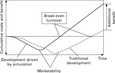
5.11 Advantage of process development by simulation vs. conventional methods. (adapted from Lemon, 2011)
5.6 Applications of computational fluid dynamics to textile technology
CFD is used in a wide range of applications, including the following:
• Air- and spacecraft: new aircraft designs are modelled in order to decrease fuel consumption.
• Automotive: improvement of the aerodynamical properties of new car bodies, simulation of fuel injection and modelling of car interior to increase passenger comfort.
• Medical: inhalation processes are analysed in order to minimize the effect of surgical operation on the patient, flow simulation of heart pumps show areas where unwanted depositions can occur which can be fatal.
• Chemical: processes in reactors are optimized with regard to reaction speed and energy consumption.
• Air conditioning: comfort of human beings in a room can be enhanced by optimizing heat distribution and air humidity.
• Process engineering: improving mixing processes, e.g. homogenization and deposition of substances.
• Maritime: development of new propeller systems to reduce energy consumption.
• Energy: increasing efficiency by better design of, e.g. windmill blades, combustion chambers.
• Sports: effects of biological examples are transferred into textiles, e.g. shark skin effect on a swim-suit, knob-structured golf balls.
In textile technology today, computational fluid dynamics is widely used to analyse processes where fast moving fibres and yarns or fabrics are involved (Martens et al., 2009). Typical examples are air-jet texturing, air-jet spinning, air-jet weaving and a range of finishing processes. Most of these processes were developed well before CFD could be used. Hence, it is now possible to directly improve existing technologies by literally taking a closer look which was unthinkable only 15 years ago. Figure 5.12 shows that, prior to 1998, there were no papers on record in the compendex database, but there has been a steady increase in the number of publications over the last 5 years. However, the overall number is still comparatively low compared with other simulation techniques described in Chapters 2–4. In this section, if not otherwise stated, all results were achieved by or under the supervision of the main author of this chapter, Ph. Jungbecker.

5.6.1 Melt-spinning
Melt-spinning is widely used to produce synthetic fibres and yarns, e.g. from polyester and polyamide. Granulate is molten by an extruder, the molten mass pumped through the spin pack, distributed onto a large number of capillaries and spun into single filaments before they are quenched, drafted and wound up onto bobbins. CFD can be applied to several components of this process. A typical application is the spin pack, where the current of the polymer can be analysed in order to avoid dead water areas in which the polymer flow is subjected to different and hence undefined conditions. This could lead to different properties of the filaments which may go unnoticed up until the final stages of the textile process chain, e.g. finishing and dyeing. In the production of spun-bonded nonwovens, several thousands of filaments are produced by one spinneret. Modelling the behaviour of the polymer flow inside the spin pack can significantly reduce costs by increasing quality of the product (Jungbecker et al., 2009). Plate III shows the flow lines of a polymer inside a bicomponent spin pack. The distribution of the polymer inside the capillaries can clearly be seen.

Owing to the visco-elastic properties of the polymer, a widening and thus a distortion of the filaments can occur when the polymer leaves the spinneret. A modelling of this process using CFD can help to achieve the desired filament cross-sections. The quenching process of the filament process is determined by heat transfer inside the yarn and heat transport outside the yarn. By applying CFD, it is possible to analyse this process and thus to optimize it, which cannot be achieved by pure measurement as this does directly effect the quenching itself.
5.6.2 Melt-electrospinning
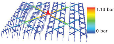
Electrospinning has been used since the 1920s but has not yet been commercialized on an industrial scale. A polymer is melted, filled into a syringe and injected into an electrical field where the fibres are drafted. With this process, fibre diameters below 500 nm can be realized which is not possible with conventional processes. A CFD simulation was employed in order to upscale the process to commercial throughput (Hacker et al., 2009). Based on these results, a new spin pack design was realized which had an even distribution of the polymer melt and low residence times. This improved the fibre quality considerably. By analysing the temperature gradient directly underneath the spinneret, it is now possible for the first time to produce nano-fibres in a continuous process. Plate IV shows the pressure distribution inside the spin pack (left) which led to the design of a new spin pack.
5.6.3 Drafting of filaments
Drafting processes are common in many fibre and yarn manufacturing processes. The filaments are normally heated to temperatures above glass transition point, thus allowing easy drawing. By applying CFD to analyse the heat loss in draft zones, it was possible to identify the weak spots in a typical drafting machine and hence to redesign it in order to reduce energy consumption and to equalize the drafting conditions. The new design was put into practice (Plate V) and measurements showed that the energy consumption could be reduced by up to 30% owing to the new design.
5.6.4 Air-jet texturing
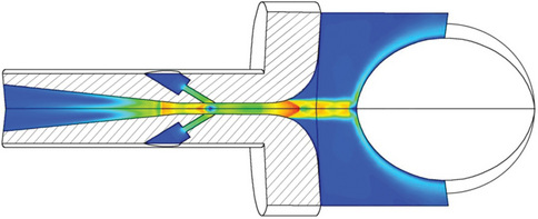
Air-jet texturing is a process to improve the handling of flat yarns made of synthetic fibres. The yarn is guided through ceramic jets and subjected to pressured air. This results in a supersonic flow inside the jet and an impulse wave at the outlet. CFD was used to analyse the current, which provided an insight into the flow inside the jets which is not possible with conventional measuring technology. Plate VI shows a typical flow inside and outside of the actual air-jet.
5.6.5 Card
In a card, fibres are parallelized, cleaned and a sliver is formed. The main components of a card are the licker-in drums, the swift, the carding elements and the doffing cylinder. Owing to the small distances between those fast rotating elements, there are strong air flows by which the fibres are affected considerably during carding. Since space is limited, the use of measuring devices is confined to certain areas where they do not have an impact on the actual process. The application of CFD to model the currents inside the card is therefore an interesting approach to analyse and hence improve the carding process (Seide et al., 2008). Plate VII shows the drag flow between swift and the slowly rotating doffing cylinder. The simulation results show that this current is directly affected by the distance between swift and doffing cylinder, the carding cloth and the velocities of the components. By adjusting the respective parameters, it is hence possible to improve the carding process.

Plate VII Air flow inside a card (left: between swift and doffing cylinder, top: between carding elements and swift).
Han et al. (2009) analysed the air flow between back plate and swift by applying CFD. They found that the static pressure increases to its maximum value near the inlet and decreases towards the outlet along a zone between back plate and swift. A comparison of the simulation results with experimental data showed a good correlation. A practical application was not given.
5.6.6 Staple fibre spinning
Zou et al. (2009) analysed the air flow in the condensing zone of a compact spinning device with a perforated drum (Fig. 5.13). By modelling the trajectory of single fibres applying CFD, it was possible to determine the parameters affecting the condensing mechanism. The trajectories were calculated by having single fibres starting from different positions of the last drafting roller. Firstly, the forces on an individual fibre were calculated. This led to the accelerations of the fibres and the respective velocities. They were used to calculate the displacements in all three dimensions and hence the trajectories of the fibres. For the model, it was assumed that the air flow is viscous and incompressible and the process adiabatic.

5.13 Condensing zone of a compact spinning device. (adapted from Zou et al., 2009)
Rengasamy et al. (2008) investigated the influence of an air-jet on ring spinning with regard to hairiness. They assumed the air flow to be viscous and compressible and the process to be adiabatic. The results in terms of air velocity and drag forces acting on the fibres showed the influence of the axial angle of the air inlets of the nozzles on yarn hairiness. They correlated well with measured values.
Zeng and Yu (2003) analysed the air flow in the nozzle of an air-jet spinning machine. They determined the resulting air flow when changing nozzle pressure, jet orifice angle and jet orifice position. A higher nozzle pressure led to higher axial and tangential velocities of the fibres and subsequently to better tensile properties. The influence of the jet orifice angle is complex and was not clearly visible. The position of the jet orifice did not considerably affect the air flow pattern. In a follow-up paper, they used the results to simulate the motion of fibres inside the nozzle using a two-dimensional model (Zeng and Yu, 2004). A comparison with photographs taken by a high-speed camera showed a reasonable correlation to the theoretical results. Zhu et al. (2008) developed a three-dimensional CFD model of the flow field inside the nozzle of a murate vortex spinning machine. No verification with experimental data was given.
In a paper by Morimoto et al. (2010), the currently used design of a nozzle for Murata vortex spinning is analysed applying a two- and a three-dimensional CFD approach. Different nozzles were investigated and produced so that theoretical and practical results could be compared. It was found that the currently used nozzles are suitable to produce vortex yarns which did not come as a surprise.
An interesting paper on friction spinning was published by Ishtiaque et al. (2010). The authors design a CFD model to analyse the air flow inside the transport duct of a DREF-III friction spinning machine. After specifying the boundary conditions, e.g. geometry of inlet, outlet and moving wall, pressure and velocity distribution were calculated by applying the k-e model for turbulent flow. After a thorough investigation of the influencing parameters, they simulated the effect of additional slots in the duct on air pressure and velocity in order to reduce the turbulence and hence to improve the yarn quality. The results are shown in Plates XIII and IX. The effect of the slots on the turbulence of the flow is apparent. A practical test with a modified duct showed that the yarn properties could indeed be improved with this measure. This is an excellent example of a CFD simulation that was actually used to improve machine design.
5.6.7 Fabric production
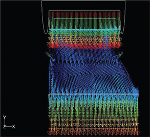
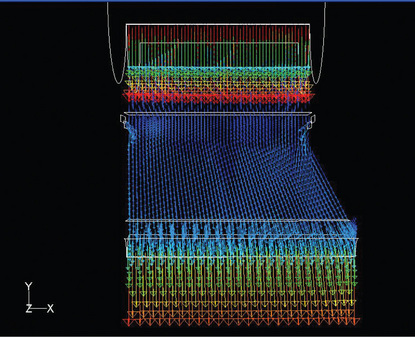
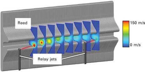
For many kinds of fabrics, air-jet weaving is a very economical process due to its high production speed. A major disadvantage is the high cost for the pressured air which is required for the weft insertion. The instationary flow field during weft insertion was analysed using CFD by Jungbecker et al. (2011). The results of the analysis can then be used to significantly decrease air consumption without affecting the machine efficiency. The weft insertion components comprise main jets in tandem configuration, a large number of relay jets, e.g. 52, and the reed which in turn consists of, for example, 4200 dents.
The geometric complexity makes it impossible to simulate one single CFD model to calculate the instationary flow field. Hence, developing a simplified model which does not affect the simulation results too much is unavoidable. In a first step, main jet, relay jets and reed are considered independently of each other which allows designing a highly accurate model for each component. In a second step, these models are simplified and new models are designed. The results of the respective simulations are then compared with the results of the detailed simulations of the first step until they coincide sufficiently well. In a third step, the whole weft insertion process is simulated taking into account the findings of the previous steps.
The results of the flow simulation show that a major part of the usable flow energy is lost during the detonation shocks of the relay jets. Air arriving at the reed channel flow backwards out of the channel and is hence lost. In other simulations, the yarn behaviour during weft insertion was analysed based on the previous findings. By changing the relay jets' turn-off times from a linear to a parabolic profile where the relay jets in the middle section are turned off earlier, it was possible to reduce pressured air consumption by 30% for a prototype weaving machine and by 10% for a commercially used weaving machine. Plate X shows the three-dimensional air flow in the reed channel.
Belforte et al. (2009) studied the flow field inside an air-jet loom main nozzle by applying a two-dimensional CFD model. They designed different models and compared the simulation results with experimental data in order to find the best-fit model. Then they analysed the influence of the length, shape and size of the acceleration tube on the yarn drag force. This led to an optimum value of the acceleration tube length for which the drag force on the yarn can be maximized.
6.6.8 Permeability of fabrics
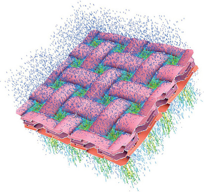
The permeability of textiles is of great interest for a wide range of applications where air or fluids flow through textile structures. Typical examples are outdoor clothing and textile preforms for composite production. A CFD simulation can be used to predict how the infusion resin spreads inside the structure and whether air inclusions occur. Plate XI shows a typical example for a multi-layered braided structure which is used for a ceramic-fibre reinforced aluminum part.
The flow of the resin through a carbon fibre fabric for use in composites was analysed by Zeng et al. (2010). They designed a unit cell to represent the three-dimensional woven fabric geometry from a set of experimentally determined geometric parameters. The calculated through-thickness and in-plane flow was then compared with actual results. The correlation was found to be satisfactory. Then, the influence of fabric geometry on permeability was analysed and it was found that the weft yarn cross-section has the largest effect.
5.6.9 Heat resistance of fabrics
A mathematical model to determine the thermal resistance of woven fabrics was designed by Kothari and Bhattacharjee (2008). They regarded the yarns, intersections and air pores of a fabric as a system of resistances. The authors assumed the woven fabric to have a cellular geometry through which conductive heat transfer occurs from the air pores as well as the yarns. Hence, all basic weaves can be regarded as modifications of a simple geometry of air pores, yarn sections and intersections. The yarns were considered to be porous and comprising infinite cylindrical fibres and air. Heat transfer through convection was neglected but was included in the CFD model in part 2 (see below). Heat transfer by radiation is considered. The underlying model is explained in great detail and could possibly serve as an example for other similar applications. The predicted and the measured values coincided very well which proves the viability of this approach.
In part 2 of the publication (Bhattacharjee and Kothari, 2008), this model was used as the basis of a CFD simulation which also included heat transfer through convection and a wind tunnel simulation. Forced convection was accurately represented by the model, natural convection could not be modelled to the same extent. This publication is recommended reading for any user wishing to simulate heat transfer through textiles by applying CFD. Another CFD-based simulation of the permeability of multifilament woven fabrics was developed by Wang et al. (2006). The results are compared with those from another analytical model and show good correlation.
Hjohlman and Andersson (2009) used a CFD simulation to predict the flame spread in textile materials. One model was used to analyse the pyrolysis of the material, the other to simulate flame spread over a surface. The results were then compared with experimental data. Although there was a large difference, especially in the calculated and the actual heat release rate, the model could still accurately predict the rating of the textiles according to the European building product classification system EN 13501.
5.6.10 Nonwovens
Nonwovens made of staple fibres can be manufactured using an aerodynamic process which dissolves the material to single fibres. They are transported in an air flow onto a sieve where they form a web. The air flow is a crucial component with regard to the quality of the web. Due to their inertia and turbulences, the fibres follow the air current only partially, resulting in different trajectories of the fibres and hence in an uneven web. A model of the air flow was created without fibres which formed the basis for a simulation of the fibres. For a high fibre content (exceeding 5%), the air current can be modelled in connection with the fibre trajectories. This allows analysing the repercussions of the fibre movement onto the air flow. A simple and effective approach to simulate the fibre bundles is to consider them as spheres. Diameter and density of the spheres can be adjusted so that their aerodynamical properties resemble those of fibres. Plate XII shows the air flow and the fibre trajectories for this aerodynamical nonwovens process.

Plate XII Simulated air flow (left) and fibre trajectories (right) for an aerodynamical nonwovens process.
The mixing process used to disperse synthetic fibres in the wet-lay process was modelled by Ramasubramanian et al. (2010). A multiple reference frame model and a standard k-ε turbulence model were employed. After obtaining a converging solution for the mixing tank with water, a discrete phase model was designed by injecting spherical particles into the flow. The results obtained from the simulation and measured values coincided very well qualitatively. The CFD model can hence be used to optimize the mixing tank design for this process.
5.6.11 Finishing
Schmidt et al. (2009) analysed the commonly used blade coating process with a CFD simulation. One of the main findings was that pressure decreased with viscosity in the coating material in the area underneath the blade's edge. This is due to the geometry of the blade and can be used to optimize it. Hence, a deeper understanding of the rheological behaviour of the coating material can help to improve this process that is normally used to produce technical textiles. Other interesting papers include Menshutina and Kudra (2001), which presents a CFD based model for textile drying processes and Scharf et al. (2002), which deals with textile dyeing processes.
Yarns can be dyed in a continuous process or discontinuously on bobbins. In the latter case, the yarn is wound onto perforated plastic cones and the dye liquor flows through the material. Flow velocity decreases from inside to outside as the diameter increases. This effect was analysed using a CFD model. This approach can also be used to determine the perfusion through the bobbin for different yarn densities across the cone. As shown in Plate XIII, especially the areas close to the edges are critical as yarn density is higher and the dye liquor leaves the bobbin tangentially.

With rising energy costs and the demand for an environmentally friendly production of textiles, an efficient drying of textiles becomes an increasingly important issue. Textiles can be dried using convection, e.g. in a stentering frame, infrared radiation and microwaves, or by contact drying with rollers. Especially for convective drying processes, a simulation of the flow can help to homogenize the air flow and thus increase the process efficiency. Not only flow velocities can be determined but also relative air humidity and water vapour intake of the textiles across the dryer's cross-section. This can lead to lower energy consumption and to better product quality.
5.7 Practical advice in applying computational fluid dynamics
• Aim of the simulation: it is important to define the aim of the simulation before designing the respective model as a model can never mirror reality in all aspects. By describing the target, both, researcher and customer, know what to expect. If certain effects are to be included, the respective models need to be activated in the software.
• Boundary conditions: the result of the simulation is strongly affected by the chosen boundary conditions. Choosing wrong or imprecise boundary conditions can lead to large differences between simulation result and reality. If that happens, a sensitivity analysis of the boundary conditions is recommended. It will show whether and to what extent an error in the initial conditions does affect the simulation result.
• From simple to complex model: it is strongly recommended to begin with simple models before proceeding to more complex algorithms. If too many parameters are changed at once, it is hard to tell the effects of each parameter. A coarse discretization keeps computing time at a minimum. Hence, effects of different models on the result can easily and quickly be recognized and one does not lose precious time. Models based on discretization accuracy, e.g. for turbulent currents, are exceptions: here. It can be sensible to first test the respective models on a simple geometry before applying them to more complex geometries.
• Model simplification: simple models are preferable over mirroring a process in all details. A typical example are textiles: in a detailed simulation, the perfusion can be analysed for a small area on microscopic scale. The resulting dependency between mean velocity and pressure loss can be represented by a porosity model according to Darcy (1856). For the subsequent simulations on macroscopic scale, the textile can then be regarded as an unstructured area with a velocity-dependent impulse sink.
• Cross-linking: if possible, the use of hexaeder cells is highly recommended. Having the same edge length as tetraeder cells, 87.5% fewer cells are needed. The relation between cross-linking effort and simulation costs should be considered. With powerful hardware and a simple model, in many cases, a fine cross-linking (small mesh size) should be chosen. Especially for instationary processes and parameter studies, it can pay off quickly if the cross-linking parameters are adjusted manually.
• Validation: it is advised to check the results for plausibility already after only a few iteration steps. In particular, the magnitude order and the correct flow direction should be checked.
• Final analysis: a final analysis and interpretation of the results should never be carried out before the results are converging.
5.8 Summary
Computational fluid dynamics is a very powerful tool to simulate currents with fibres and yarns as well as flows through and around textiles. In contrast to the methods described in Chapters 2–4, however, it is essential to acquire a deeper insight into the theoretical background behind the various mathematical models, e.g. fluid mechanics, before starting to create CFD-based models and simulations. Existing software is often very complex to use and hence requires extensive experience to apply it properly. CFD is therefore not a quick-and-dirty approach to solve fluid-related problems but often a time-consuming and thus costly process. Nevertheless, CFD simulation can lead to an insight into the relation of parameters that could otherwise not be analysed. Today, its use is wide spread and has led to a considerable number of machine optimizations in textile technology ranging from fibre and yarn manufacturing to fabric production and finishing.
5.9 Web references for software tools
A site dedicated to collecting and sharing information, successful applications and software tools about CFD is:
In the 'Codes' section of the wiki on this website, interested readers can find an extensive list of free and commercially available software packages to carry out CFD simulations. This includes, besides the actual modelling and simulation software, also grid generation as well as visualization tools. As far as the authors know, this is the most comprehensive list in this respect on the internet. Hence, there is no need to give a separate list of recommended software in this section.
5.9 References
Abbot, M.B., Basco, D.R. Computational Fluid Dynamics: An introduction for engineers. Wiley; 1989.
Baliga, B.R., Patankar, S.V. New finite-element formulation for convection-diffusion problems. Numerical Heat Transfer. 1980; 3(4):393–409.
Belforte, G., Mattiazzo, G., Viktorov, V., Visconte, C. Numerical model of an air-jet loom main nozzle for drag forces evaluation. Textile Research Journal. 2009; 79:1664–1669.
Bhaskaran, R., Collins, L., Introduction to CFD Basics. Cornell Univ. 2008 http://courses.cit.cornell.edu/fluent/cfd/intro.pdf [(accessed 20 April 2011)].
Bhattacharjee, D., Kothari, V.K. Prediction of thermal resistance of woven fabrics. Part II: heat transfer in natural and forced convective environments. Journal of the Textile Institute. 2008; 99(5):433–449.
Cebeci T., Shao J.P., Kafyeke F., Laurendeau E., eds. Computational Fluid Dynamics for Engineers: From panel to Navier–Stokes methods with computer programs. Springer, 2005.
Courant, R., Friedrichs, K., Lewy, H. Über die partiellen Differenzengleichungen der mathematischen Physik. Mathematische Annalen. 1928; 100(1):32–74.
Darcy, H. Les Fontaines Publiques de la Ville de Dijon. Dalmont; 1856.
Hacker, C., Jungbecker, P., Gries, T., Thomas, H. Mehrdüsen-Elektrospinnen aus der Polymerschmelze – Die Entwicklung zum Upscaling. Proceedings of 12, Chemnitzer Textiltechnik-Tagung. 2009; 32–35.
Han, X.-G., Sun, P.-Z., Zhao, Y.-P. Analysis of static pressure in area between back plate and cylinder of a carding machine with CFD. Journal of Donghua University. 2009; 242–246.
Hirsch, C., 2nd ed.. Numerical Computation of Internal and External Flows: Fundamentals of computational fluid dynamics; vol. 1. Elsevier/Butterworth-Heinemann, 2007.
Hjohlman, M., Andersson, P. Flame spread modelling of complex textile materials. Fire Technology. 2009; 47:85–106.
Hussein, H.J. Measurements of Turbulent Flows with Flying Hot-wire Anemometry. American Society of Mechanical Engineers Fluids Engineering Division (Publication) FED. 1990; 97:77–80.
Ishtiaque, S.M., Singh, S.N., Das, A., Mittal, S., Dave, V. Optimisation of fluid flow phenomena inside transport duct of a DREF-III friction spinning machine. Part III: CFD approach. Journal of the Textile Institute. 2010; 101(10):906–916.
Jungbecker, P., Hacker, C., Gries, T., Thomas, H., Möller, M. Melt-electrospinning of nano-nonwovens. Chemical Fibers International. 2009; 59(4):228–229.
Jungbecker, P., Schenuit, H., Holtermann, T., Seide, G., Gries, T. Reduction of energy consumption in air-jet weaving. Melliand International. 2011; 17(1):32–33.
Kothari, V.K., Bhattacharjee, D. Prediction of thermal resistance of woven fabrics. Part I: mathematical model. Journal of the Textile Institute. 2008; 99(5):421–432.
Lai, M.-C., Peskin, C.S. An immersed boundary method with formal second-order accuracy and reduced numerical viscosity. Journal of Computational Physics. 2000; 160(2):705–719.
Launder, B.E., Spalding, D.B. Numerical computation of turbulent flows. Computer Methods in Applied Mechanics and Engineering. 1974; 3(2):269–289.
Lehmann, B. Large-Eddy interpretation of LDA results obtained by conditional seeding in a circular jet. Advances in Turbulence. 1988; 2:102.
Lemon, J. Why simulation should drive product development, 2011. http://www.iti-global.com/Education/Articles/SimLedDev.htm [(accessed: 20 April 2011).].
Löhner, R. Applied CFD techniques: An introduction based on finite element methods, 2nd ed. Wiley; 2008.
Marheineke, N., Wegener, R. Modeling and validation of a stochastic drag for fibers in turbulent flows. Berichte des Fraunhofer ITWM. 172, 2009.
Martens, S., Jungbecker, P., Seide, G., Gries, T., Fostering energy efficiency in textile machinery by flow simulation. B., Küppers. Proceedings of the 3rd Aachen-Dresden International Textile Conference, 2009:1–7.
Mason, W.H. Introduction to computational fluid dynamics. Applied Computational Aerodynamics. 1998; 2:8.
Menshutina, N.V., Kudra, T. Computer aided drying technologies. Drying Technology. 2001; 19(8):1825–1849.
Menter, F.R. Two-equation eddy-viscosity turbulence models for engineering applications. AIAA Journal. 1994; 32(8):1598–1605.
Morimoto, K., Tada, Y., Takashima, H., Minamino, K., Tahara, R., Konishi, S. Micro spinning nozzle having 3D profile for fiber generation with spiral air flow. proceedings of IEEE International Conference on Micro Electro Mechanical Systems (MEMS), 2010:244–247.
Peiro, J., Sherwin, S., Finite difference, finite element and finite volume methods for partial differential equationsYip S., ed. Handbook of Materials Modeling. Vol. 1.: Methods and models. Springer:, 2005:1–32 http://www2.imperial.ac.uk/ssherw/spectralhp/papers/HandBook.pdf [(accessed: 21 April 2011).].
Raffel, M., Willert, C., Wereley, S., Kompenhans, J. Particle Image Velocimetry − A practical guide. Springer; 2007.
Ramakers, R. Systematische Entwicklung von sensorbasierten OnlineÜberwachungssystemen für die Filamentgarnverarbeitung', doctoral thesis. Shaker: RWTH Aachen; 2005. [2005].
Ramakers, R., Besen, A., Gries, T. Konstruktionskatalog Sensortechnologie für die Online-Überwachung von Produktionsprozessen. Shaker; 2006.
Ramasubramanian, M.K., Shiffler, D.A., Jayachandran, A. A computational fluid dynamics modeling and experimental study of the mixing process for dispersion of synthetic fibers in wet-lay forming. Tappi Journal, p.. 2010; 6–13.
Rengasamy, R.S., Patanaik, A., Anandjiwala, R.D. Simulation of airflow in nozzle-ring spinning using computational fluid dynamics: study on reduction in yarn hairiness and the role of air drag forces and angle of impact of air current. textile Research Journal. 2008; 78:412–420.
Rodi, W., Spalding, D.B. Two-parameter model of turbulence, and its application to free jets. Waerme-Stoffuebertrag Thermo-Fluid Dynamics. 1970; 3(2):85–95.
Roller, S., Ferch, M., Munz, C.-D., Dumbser, M., Numerische Grundlagan: Finite Differenzen, Finite Elemente, Finite Volumen. Höchstleistungrechen-zentrum Stuttgart. 2005 https://fs.hirs.de/projects/par/par_prog-ws/2005D/cfd-05-be.pdf
Salari, K., Roache, P.J., Wilcox, D.C. Numerical Simulation of Dynamic Stall Using the two-equation k-ω turbulence Model. American Society of Mechanical Engineers, Fluids Engineering Division FED. 1994; 196:1–7.
Scharf, S., Cleve, E., Bach, E., Schollmeyer, E., Naderwitz, P. Three-dimensional flow calculation in a textile dyeing process. Textile Research Journal. 2002; 72:783788.
Schmidt, M., Schloßer, U., Schollmeyer, E. Computational fluid dynamics investigation of the static pressure at the blade in a blade coating process. textile Research Journal. 2009; 79:579–584.
Seide, G., Jungbecker, P., Gries, T. Simulation of staple fiber kinematics in a turbulent air stream. Melliand International. 2008; 14(1):22–23.
Wang, Q., Maze, B., Vahedi Tafreshi, H., Pourdeyhimi, B. A note on permeability simulation of multifilament woven fabrics. Chemical Engineering Science. 2006; 61:8085–8088.
Zeng, Y.C., Yu, C.W. Numerical simulation of air flow in the nozzle of an airjet spinning machine. Textile Research Journal. 2003; 73(4):350–356.
Zeng, Y.C., Yu, C.W. Numerical simulation of fiber motion in the nozzle of an air-jet spinning machine. Textile Research Journal. 2004; 74(2):117–122.
Zeng, X.S., Endruweit, A., Long, A.C., Clifford, M.J. CFD flow simulation for impregnation of 3D woven reinforcements. Proceedings of the 10th international conference on textile composites. 2010; 455–462.
Zhu, Y.D., Zou, Z.-Y., Wu, J.-M., Xue, W.-L., Cheng, L.-D. Characterizing and analyzing the airflow field inside the nozzle block of murata vortex spinning. Journal of Donghua University. 2008; 670–675.
Zou, Y.Z., Cheng, L.D., Hua, Z.H. A numerical approach to simulate fiber motion trajectory in an airflow field in compact spinning with a perforated drum. Textile Research Journal. 2009; 80(5):395–402.