
Simulation of fibrous structures and yarns
Abstract:
This chapter discusses several models which describe the mechanical properties of staple fibre yarns. Starting with definitions of yarns and their structure, a simple model of a yarn is developed. This is then used to describe the packing density of a yarn and the maximum twist it can bear without coiling. The model is then applied to determine the tensile force utilization coefficient. Finally, a theoretical model based on Koechlin’s concept is used to determine a suitable yarn twist. Applying Hamburger’s theory, a model is described that allows calculation of the mechanical properties (tenacity, breaking strain, etc.) of staple fibre yarns.
7.1 Introduction
Fibre to yarn conversion is based on two basic technology steps: spinning preparation and the actual yarn formation process. The properties of the yarns spun by various technologies depend on the yarn forming process and the level of the fibre arrangement. Twisted yarns are a special type of fibrous assembly. Whole yarns can be intuitively divided into two parts − core and cover. The core is the sphere near the yarn axis, where the fibres are well arranged and the packing density is relatively high. The cover (characterized by fibre hairiness) comprises ends, loops and other fibre segments with a lower packing density. Strict boundary lines between these two spheres do not exist. The yarn diameter is placed in this intermediate layer, making its accurate determination difficult.
A helical model (see Section 7.6) is usually used to describe an idealized fibre assembly in the yarn structure. During twisting of the yarn, some fibres are displaced from their central position to the yarn surface (migration effect). Structural and mechanical parameters depend on the fibre arrangement. Mechanical parameters are related to the fibre arrangement in the yarn core. The degree of hairiness is determined by the fibres’ configuration on the outer layer of the yarn. Yarn unevenness is connected to the distribution of the fibres in the whole yarn.
7.2 Fibres and yarns: definitions and factors affecting quality
Yarn quality depends on the types of fibre (fineness, diameter, shape factor, length, flexural rigidity, torsion rigidity, tenacity, extension to break, friction, crimp and compression resistance), the geometrical parameters of the yarn (twist, count, blending ratio − migration effect), the technology of production (classical or innovative, production rate, cost of yarn, end purpose of yarn, setting of production line) and quality control (testing of randomly selected yarn samples, systematic analysis of yarn production).
Staple fibres are the fundamental units of yarns. Any yarn model must include the required parameters of fibres (Fig. 7.1) and their relationships. Some of them are introduced here. One of the most frequently used fibre parameters is fibre fineness − the ratio between fibre mass and fibre length. The main physical unit of fibre fineness is 1 tex, which is equal to 1000 m of a fibre/yarn weighing 1 g. For fibres, the unit dtex is often used, which is equivalent to 1 g/10 000 m. Typical values for micro-fibres are below 1 dtex, for cotton fibres around 1.6 dtex, for wool often around 3.5 dtex and for coarse carpet fibres above 7 dtex.
From a geometrical standpoint, fibre ‘fineness’ is characterized by the ratio between volume V and length l, but standard fineness is also influenced by the fibre density ρ. Therefore, it is not correct to compare the finenesses of fibres having different densities solely by their standard fineness; it is better to use the ratio t/ρ. Fineness and density define the cross-sectional area of a fibre:
The calculation of the cross-sectional area allows evaluation of the equivalent fibre diameter as shown in Fig. 7.2. For cylindrical fibres, the derivation is trivial. For non-cylindrical fibres, the same equation represents the diameter of a ring having the same cross-sectional area.

The equivalent fibre diameter d is hence given by:

The perimeter of a non-cylindrical fibre is always larger than the perimeter of a ring having the same cross-sectional area. In this context, the fibre shape factor q, according to Malinowska (1975) is illustrated in Table 7.1.
Table 7.1
Values of shape factor for various fibres
| Shape of fibre cross-section | q |
| Circle – ideal |
0 |
| Circle – real | 0 to 0.07 |
| Triangle – ideal |
0.29 |
| Triangle – real | 0.09 to 0.12 |
| Mature cotton | 0.20 to 0.35 |
| Irregular saw | > 0.60 |
If we know the (typical) shape factor of a fibre in advance, its perimeter p can be calculated with Equation [7.3].
Many important properties of textiles (especially transport of moisture) depend on the total area of the fibrous surface A. Therefore, it is very useful to know the surface area per unit mass of fibrous material a. The derivation of the so-called specific surface area is shown here. (Note: we can neglect the topmost and bottommost cross-sectional areas of fibres because, as the fibres are very long, these two areas are relatively small − e.g. 0.025%.) The specific area can be calculated according to
The physical definition of the mechanical (normal) stress is the ratio of force F and the corresponding area s measured in [MPa].
The term stress in textiles, the ratio of force and the corresponding fibre fineness is measured in [N/tex], [cN/dtex] and also called ‘breaking length km’:
It is apparent that it is not correct to compare stress or strength of fibres having different densities by using the standard textile units (e.g. N/tex, breaking length km). Typical values for cotton, PET and steel are given in Table 7.2.

7.3 Fibrous assemblies: volume, density and mass
Inside a textile fibrous assembly (Fig. 7.3) there is the fibre volume V. The total volume of this body is called Vc. The compactness of this body is characterized by the ratio between these two volumes and is known as the fibre packing density μ (equation [7.9]). Alternatively, this value is called packing ratio or volume fraction. The fibre packing density value lies in an interval from 0 to 1. With the volume of fibres V and the total volume Vc including air, we have:

7.3.1 Compactness of fibrous assemblies − fibre packing density μ
The fibre packing density μ is defined by:
Table 7.3 gives typical values of the fibre packing density for different materials. (Note: the packing density values around 0.4 to 0.5 are specific just for twisted staple yarns and practically no other fibrous structures have this value. Therefore, the yarns represent very specific types of fibrous assemblies.) Table 7.3 lists typical values of the packing density for various fibrous assemblies.

7.3.2 Areal interpretation
In a very (elementary) flat box as shown in Fig. 7.4, the lengths of the fibre sections inside this box are short; hence they can be interpreted as straight abscissas. It is now possible to derive the total volume and the volume of fibres according to:

where S is the total sectional area of all elements as shown in Fig. 7.4. Hence we get
The fibre packing density of the flat box is then defined as the ratio between two areas. (Note: the fibre packing density in yarn is often expressed as the ratio between two cross-sectional areas.)
7.3.3 Mass interpretation
Yarn mass is based on density. The mass of a fibrous assembly is given by the mass of the fibrous material only. Using the total volume of the fibrous assembly, the density of the fibrous assembly can be defined. Using only the volume of fibres, the density of fibres can be derived. The fibre packing density is then given by the ratio between these two densities:
with ρ* standing for the density of fibrous assembly and p as the density of the fibre material.
7.4 Yarn parameters: fineness, density, diameter and twist
Twisted staple yarn is a special type of fibrous assembly. For its description we use quantities as shown in Fig. 7.5. The yarn fineness (‘yarn count’) is one of most important standard values, but it is not sufficient to describe a yarn structure properly. The ratio between fibre volume and unit length characterizes the yarn ‘size’ geometrically well, but the yarn fineness is moreover influenced by the fibre mass density. Therefore, it is not possible to compare the yarns from different fibres using yarn ‘count’ (e.g. cotton and PET yarns). In this case, only ratios of yarn count to fibre mass density can be compared.

7.4.1 Yarn fineness
Fibre fineness in [tex] is defined as:
Figure 7.6 shows an elementary short part of a yarn. The sum of the areas of all fibre sections in yarn cross-section is called the substance cross-sectional area of the yarn. The substance cross-sectional area of yarn is equal to the ratio yarn count to fibre mass density, or fibre volume per unit length of yarn.

Definition of substance cross-section area is:
If the yarn is compressed, all air is removed from the inside of the yarn. Then, the yarn cross-sectional area is equal to the substance cross-sectional area and hence the compressed yarn will have the substance diameter according to Fig. 7.7.

7.4.2 Substance diameter
The substance diameter can then be calculated according to:

(Note: the diameter of real yarn is always bigger than the substance diameter.)
7.4.3 Relative fineness
The ratio of yarn fineness (count) to fibre fineness is another important quantity and is called the relative fineness of yarn. It is given by
(Note: this value is not identical to the number of fibres in the yarn crosssection.)
7.4.4 Coefficient kn
The fibre sectional area is a function of the fibre slope, as shown in Fig. 7.8. The coefficient kn is the ratio between the fibre cross-sectional area and the mean fibre sectional area. Taking into account the fibre geometry according to

The value kn is the weighted harmonic mean value of cosines of the slope angles. If each angle is equal to 0, we have kn = 1. This configuration corresponds to the parallel fibre bundle.
7.4.5 Number of fibres in the yarn
The number of fibres in the yarn can be determined by
The coefficient kn is related to the relative fineness and the number of fibres according to equation [7.29]. (Note: beyond the scope of a parallel fibre bundle, the number of fibres in the yarn cross-section is always smaller than the relative yarn fineness.) Equation [7.29] also enables us to determine the coefficient kn experimentally.
7.4.6 Packing density of a yarn
According to equation [7.9], the packing density of the yarn is given by
Inserting the substance diameter from equation [7.19], we have
If the packing density is known, the yarn diameter can also be determined using equation [7.33].

7.4.8 Twist intensity
Some yam characteristics are based on the yarn twist. Because the dimension of the twist Z is [m −1] and the dimension of the yarn diameter is [m], the product of DZ is dimensionless. The twist intensity is then given by
If the peripheral fibre in Fig. 7.9 follows a helical path, the twist intensity is also the tangent of angle pD of this fibre.

7.4.9 Twist coefficients
The so-called ‘twist coefficients’ (twist multipliers) create another group of twist characteristics. The first type is related to the yarn substance crosssectional area S. This coefficient is called ‘areal’ and only of theoretical value. The second type is related to the yarn fineness (count). This coefficient is commonly used in practice. General coefficients use a general value of twist exponent q. Koechlin’s coefficients use the twist exponent 0.5. These can be also written in an alternative way, equations [7.38a, b] and [7.39a, b].


(Note: the common version of Koechlin’s coefficient is usually used in spinning mills.)
7.4.10 Dimensionless quantities
The dimensionless quantities are always very interesting, because they characterize the internal relationships in material body, processes, etc.:
In place of the yarn parameters T, Z, D and n it is possible to use four of the dimensionless parameters, e.g. t, k, m and kn.
7.5 Modelling of internal yarn geometry: helical yarn model
Practical yarn properties are the result of fibre properties, the mutual fibre interactions inside the yarn, and the interactions between yarn and outer influences. The internal structure of a yarn is very important especially for the geometrical and mechanical properties of the yarn. From Fig. 7.10 it is apparent that the specific regulations of the internal yarn geometry are relatively complicated due to the complex nature of deterministic and random influences. The general fibre trajectories have complicated shapes, a random character and show deterministic trends.

7.5.1 Fibre elements
The position of fibre elements is determined by their coordinates r, φ, ζ, their length by dl, and their direction by the elementary increments of the coordinates, i.e. dr, dφ, dζ as shown in Fig. 7.11. It is important to note:
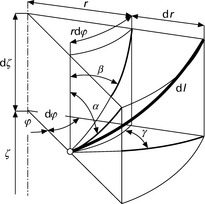
• the increment dζ is defined always as positive; and
• the positive value of the increment dζ corresponds to the sense of direction of yarn twist.
(Note: evidently, the angle b relates to the yarn twist intensity.) From Fig. 7.11, we get:
The following relations are evident from earlier equations:


Evidently, two independent values define the direction of fibre element. Those are the two ratios of increments of coordinates: dφ/dζ and dr/dζ:
where z stands for the twist of the element (which is not necessarily identical to the yarn twist Z).
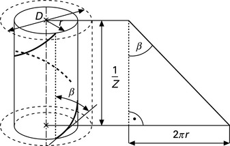
7.5.2 Helical yarn model
In a helical model, two differential equations characterize the path of each fibre:
Assuming that the fibre passes through the ‘starting point’ with coordinates (r0, φo, ζo), then we obtain by integration:

The yarn twist has a sense of constant Z. The height of one fibre coil is 1/Z and the same for all fibres. By rearrangement:
The angle β is constant at a given radius r. By integration:

The fibre lies on the same radius of the cylindrical surface. (Note: the same conclusions can be obtained from Fig. 7.12.) Assumptions of a helical model can be formulated also in the following way:
• helical paths of fibres (same sense of rotation);
• common axis of all helixes is yarn axis;
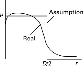
The fibre positions in the yarn (‘starting points’), which are not determined by the assumptions stated before, can be characterized by the radial function of packing density μ = μ(r) as shown in Fig. 7.13. Because it is relatively complicated, a simplifying assumption is used: the packing density must be constant in all places inside the yarn.
If all these four assumptions are valid, then this model is called an ideal helical model. Helical models and their applications are the oldest concepts of yarn modelling, associated with the scientists A. Kӧchlin (1828), E. Müller (1880), S. Marschik (1904), A.CH. Gegauff (1907), R. Schwarz (1933), E. Braschler (1935), V.I. Budnikov (1945), L.R.G.Treloar (1956) and others.
7.5.3 Number of fibres and shortening of yarn
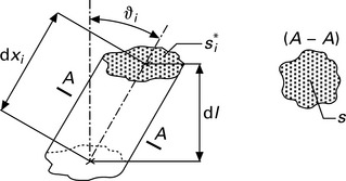
Based on Braschler (1939), a differential annulus (‘differential layer’) is created at the general radius r in a cross-section of the general helical model as shown in Fig. 7.14. The area A of the differential annulus is then given by

where dS represents the area of the fibre sections in the differential annulus (dark grey in Fig. 7.14). The area of the fibre section can then be determined by
The area of the oblique section of one fibre is then given by (according to Fig. 7.15):
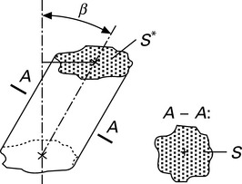
where s stands for the fibre cross-section.
The number of fibres in the differential annulus is hence
The substantial cross-sectional area of the yarn is given by
The mean packing density of the yarn is given by
The number of fibres in the yarn cross-section is then

The coefficient kn can then be determined by

In order to calculate S, μ, n and kn in a numerical simulation, the relation μ = μ(r) must be known. The function μ(r) can be obtained by experiments or by applying a theoretical model as described, e.g. in Hearle et al. (1969). A complete description of the ideal helical model can be found in Neckar and Das (2012).
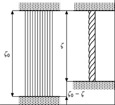
7.5.4 Yarn retraction in the ideal helical model
Figure 7.16 shows the yarn retraction in the ideal helical model. The yarn retraction can hence be calculated according to
The latent twist coefficient is then given by
where Zo = Nc/ζo, Nc stands for the number of coils per length ζ0 and T0 = m/ζo, with m representing the fibre mass. The real twist coefficient is then given by
The yarn retraction can also be calculated for an ideal helical model with

Using equation (7.39b), we can derive

Using equation (7.66), we can express 5 as a function of latent twist coefficient αo as follows:
This square equation has the solution
Since the discriminant of the equation must not be negative, we get
which means that the latent twist coefficient is limited. The limit case is given by
For this case we get from equation [7.71]: δ = 0.5.
With equation [7.68] we then get ![]() and hence βD = 70.5°.
and hence βD = 70.5°.
we get ![]() . This means that the value of the twist intensity is also limited as is shown in Fig. 7.17. Staple yarns have smaller retractions than filament yarns since fibres slip in the region around the yarn surface during the twisting process (‘false draft’) and therefore the ‘effective’ yarn diameter Dδ is smaller than D.
. This means that the value of the twist intensity is also limited as is shown in Fig. 7.17. Staple yarns have smaller retractions than filament yarns since fibres slip in the region around the yarn surface during the twisting process (‘false draft’) and therefore the ‘effective’ yarn diameter Dδ is smaller than D.
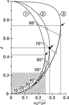
7.17 Graphical representation, curve 1, of equation [7.71]. Curves 2 and 3 are from other models of yarn retraction.
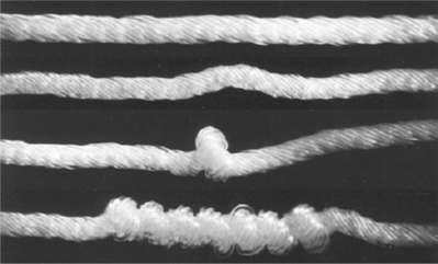
The saturated twist (limit case) can be observed experimentally, but for a smaller value of the latent twist (usually for βD from 45° to 55° in the case of filament yarns). The axial asymmetry of twisted yarn is the probable reason of this phenomenon. If the twist level exceeds the saturated twist of a yarn, this additional twist cannot be absorbed ‘inside’ its structure thus coils form (twist of the second order) as shown in Fig. 7.18.
7.6 Stress–strain relations
The general element of the helical fibre (length dl, angle β) as shown in Fig. 7.19, lying at the radius r determines an elementary cylindrical surface with certain dimensions (right, top). After the yarn has been subjected to elongation, the same element shifts itself to a new (right, bottom) position at a smaller radius' with new angle β' and new dimensions. Hence we have

The yarn axial strain is given by
The contraction ratio according to Poisson is defined as
The fibre strain can be calculated using
Based on Pythagoras’s theorem from Fig. 7.19, we have before deformation:

(Note: because of the continuity of the yarn body, dφ must be the same.) Using earlier derived equations, we obtain finally
Assuming that strains are small, we have
Note: Gegauff (1907) used η = 0 and obtained
Assuming the easiest case, that the fibre tensile stress–strain relation is linear, we get
where σ represents the tensile stress and E the Young modulus. Figure 7.20 shows the load on a helical fibre element. The axial force in the fibre is then given by

and the component force in the direction of yarn axis is
The fibre sectional area is given by
Assuming small deformations, the normal stress on this area is then given by
The fibre sectional area inside the differential annulus can be determined using equation [7.56] and then the yarn axial force is

After rearrangement and integration we get the axial yarn force
At the same strain εa, the untwisted fibre bundle of the same yarn count has the same substantial cross-sectional area and the axial force is then
The tensile force utilization coefficient in the twisted yarn is then
A graphical representation of equation [7.95] is shown in Fig. 7.21. It is important to note that φ is also applicable for the determination of filament yarn strength (by h = o.5) (Fig. 7.21).

7.21 Graphical representation of equation [7.95] and comparison with experiment results.
The strength of a staple fibre yarn can usually be interpreted as:
Figure 7.22 shows the breaking tenacity versus twist. The top curve shows the model above. The frictional effect is still an open problem to be described theoretically, hence the resulting curve is only an approximation of the real case. Note: the helical model is the best known theoretical concept to describe the internal yarn geometry. Only a few basic concepts have been described here. Many other versions and their applications can be found in traditional textile literatures. A concise summary can be found in Neckar and Das (2012).

7.7 The relationship between yarn count, twist, packing density and diameter
The relations among count, twist and diameter of a yarn are related to specific geometrical and mechanical properties of the yarn. The basic quantity behind these relations is yarn packing density. The first traditional theoretical model regarding these relations was introduced by Koechlin in 1828 (Neckář, 1990). He studied the yarns produced from the same fibrous material using the same technology for analogous end uses. At that time, the scientific knowledge about the mechanics of fibrous assembly and yarn geometry was not sufficient to create a realistic model. Hence, it was necessary to substitute the unknown relations by the first categorical assumption as shown here.
7.7.1 Theoretical model according to Koechlin's concept
The initial assumptions (problem limitation) are:
Koechlin’s first assumption
Koechlin’s first assumption (substitution of knowledge of mechanics) was that the packing density is a function of the twist intensity only:
Hence we get for the twist coefficients:
• areal Koechlin’s type (equation [7.38]):

• common Koechlin’s type (equation [7.39]):

and for the diameter multipliers, we have
• areal multiplier (equation [7.34]):
• common multiplier (equation [7.34]):
The second assumption is how the yarn is twisted. If yarns of different counts are produced from the same material using the same technology, all yarn properties should be similar. But in reality, this has proven not to be possible. Therefore, we must go ‘one step back’: what will happen if we consider only geometrically similar yarns? (Not all values, only those that are not related to fibre fineness.) Then, the other properties may be also more or less similar. In case of geometrical similarity, the corresponding angles are the same. So, the angles βD must be same and therefore the twist intensities κ must be the same too.
Koechlin’s second assumption
Koechlin’s second assumption is directed to a suitable twist. This means that the twist intensity of yarns of different counts shall be the same:
Hence we have for the twist coefficients:
For the diameter multipliers, we get
The derived equations are traditionally used in textile mills. The calculation of a suitable yarn twist is often necessary for the yarn production and the calculation of the yarn diameter is necessary for fabric manufacturing. In many cases, the resulting values are not sufficiently precise. On the one hand, the assumption about the geometrical similarity is acceptable. On the other hand, the twist intensity κ is not a function of packing density μ only as it depends also on the yarn count. Hence, the Koechlin’s first assumption is not sufficiently accurate and thus an empirical correction of Koechlin’s theory is necessary.
7.7.2 Empirical corrections of Koechlin's theory
Table 7.4 gives an overview about various twist coefficients that were determined by different authors. According to equation [7.36], a suitable yarn twist can be derived from
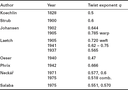
where q is an empirical value of the twist exponent with normally q > 0.5. The yarn diameter can then be calculated with
where Qa, w, v… are empirically determined values, with w > 0.5 (e.g. cylindrical yarn: w = 0.56) and v < 0 (e.g. cylindrical yarn: v = − 0.22).
The problems with models like Koechlin’s concept initiated interest for a deeper knowledge of the internal yarn mechanics and motivated researchers to think about alternative ways to solve the problems. The concept of radial forces equilibrium based on the differential equation (Hearle et al, 1969) is general, but very complicated and requires knowledge on some not yet sufficiently known inputs (e.g. stress–strain tensors relation). The model presented in the next section is ‘something in-between’. It is not as difficult as the concept of radial forces equilibrium but is sufficient for the present knowledge we have about the mechanics of fibrous assemblies.
7.8 A simple mechanical model of yarn properties
The model is based on the helical geometry of fibres inside the yarn (for assumptions see Section 7.6). A fibre coil lying on the imaginary cylinder of radius r is shown in Fig. 7.23. Unwinding the surface of this cylinder results in a triangle, whose geometry determines the fibre slope angle β. It is known from analytical geometry that the curvature of the helix is given by:

Obviously, the radius of curvature (radius of the so-called oscillating circle) is the reciprocal value of the curvature:
7.8.1 Centripetal force per unit volume of a fibre
According to Fig. 7.24, the centripetal force of a fibre can be calculated for small angles φ by

The volume of the unit is given by
where s stands for the fibre cross-sectional area. The centripetal force per unit volume of the fibre is then
7.8.2 Compressing zone
The model described here is based on the idea of a compressing zone. Around the yarn surface, the interaction of fibres is not very intensive, since no fibre in this layer is compressing from the outside. Therefore, the number of contacts, the frictional forces, the packing density and the fibre axial forces F are very small. So, the specific centripetal force P1 must also be very small. Around the yarn axis, the slope angle φ is very small. This means that the curvature of these fibres is also very small, hence the radius of curvature is very high and so the specific centripetal force P1 must be very small too. Only the compressing zone between these layers can produce a significant centripetal force P1. This leads to the assumption that the only significant centripetal force is present in the compressing zone between the layers, as shown in Fig. 7.24. The cross-sectional area of the compressing zone is given by
The total volume of the compressing zone is hence
The fibre volume in the compression zone is then
The total centripetal force in the compressing zone is hence given by
For the following conclusions, we assume that the centripetal force P acts on the cylinder at radius r, hence all partial forces at radius r are centralized (Fig. 7.25). The surface area of cylinder with radius r is given by

The pressure developed in the compressing zone is then
From equation [7.116] we get then after rearrangement

Summarizing the constant parameters with
The value C depends on the three quantities: 2r/D, σ and a/d. The position of the compressing zones may be relatively the same with regard to yarn surface cylinder and so 2r/D is perhaps constant. The axial stress s, acting on the yarn substance cross-section, is determined by the centrifugal forces and the tensioning of the fibres during twisting. This stress is perhaps constant too. It is very difficult to comment on the relative thickness of the compressing zone a/d. There is not yet a clear enough physical imagination about it, but from practical experiences this value may be considered as a constant too. (This is an open problem for the future.)
It can be assumed that the quantity C is a parameter that depends on the fibrous material and spinning technology used. The derived equation hence expresses pressure p, as a result of the yarn geometry. Simultaneously, the pressure p is a function of the packing density (compression of fibrous assembly) according to
From equations [7.122] and [7.123], we get the following equivalence:
The packing density can hence be expressed as a specific function of the yarn geometry;


depends on the material and the technology used. Hence, we get the final equation for the packing density
Note: m here is a function of ZT1/4, whereas Koechlin’s exponent is 1/2.
The parameter a in equation [7.127] is usually equal to 1 and μm is usually equal to 0.8 (influence of yarn surface). Typical values for Q are summarized in Table 7.5. Example: for carded cotton yarn of T = 29.5 tex, Z = 719.43 m −1 (a = 123.57 m −1 ktex −1/2), the right-hand side of the derived equation is 0.27016 and this corresponds to m = 0.460 on the left-hand side (calculated by numerical method). Then, the yarn diameter is D = 0.232 mm.

A problem in the practical application of this equation is the determination of the root μ. This can be solved by applying a numerical method (e.g. interval splitting method) or by approximating the value if the packing density of the yarns is around μ* as follows:
The yarn diameter can then be calculated with
with ρ[g/cm3], Q[m2 tex −0 5], T [tex], α [m1 ketx1/2].
Example: let Q = 9.61 × 10 −8 m2 tex −1/2, ρ = 1520 kg m −3 and μ* = 0.46. Then we get b = 5.11261, c = 9.70918. For an approximated μ we have
and for the approximate D we get
Experiments were undertaken on carded cotton yarns and roving (Fig. 7.26). Yarn count ranges were from 16.5 to 100 tex, twist factor ranged from 83 to 140 m −1 ktex1/2. Equation [7.125] helps in deriving the relation for a suitable yarn twist.

7.8.3 Suitable yarn twist
In order to determine a suitable yarn twist, the model described above together with a more precise form of the theory according to Koechlin is applied. The slope of surface fibres is then not characterized by the angle βD at a diameter D of the cylinder but by the slope of surface fibre axis, e.g. the angle β' at a diameter D' on the cylinder as shown in Fig. 7.27. The modified diameter D' characterizes the position of the axes of surface fibres, with D' < D. Following this we have
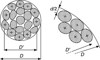
In case of the theoretical limit structure (Fig. 7.27), we have
Inserting [7.132] into [7.131] leads to


The real yarn has a diameter D and a proportionally longer modified diameter D' and therefore the value of the Schwarz constant is the same. The modified angle β' (slope of fibre axes on yarn surface) is then given by
Rearrangement of equation [7.127] leads to

In order to determine the quantity R, there are two possibilities. First, yarns are from the same material and of the same end use. Then we can distinguish between case 1 (same technology and different yarn counts) and case 2 (different technologies and same yarn count):
• For case 1, the modified angle β' (slope of axes of peripheral fibres) should be constant, hence, R = constant.
• For case 2, the contact density ν (it is valid ν. = kν.μ2) should be constant, hence μ = constant and the left part of equation [7.138] is constant and therefore R = constant.
In general, we have R = constant for all yarn counts and technologies. The parameter a in equation [7.139] is usually equal to 1 and μlim is usually equal to 0.8. Typical values for R are given in Table 7.6.
Table 7.6
| Material | ρkg m 3] | R [tex1/2] |
| Cotton − long staple | 1520 | 2.145 |
| Cotton − medium staple | 1520 | 2.737 |
| Viscose, C-type | 1500 | 4.589 |
| PET, C-type | 1360 | 3.563 |
| Wool | 1310 | 2.341 |
In order to illustrate the practical use of equations [7.127] and [7.139], we consider a typical example. Q and R are usually known (Tables 7.6 and 7.7), as are t, p as material constants and T as the required yarn count. Hence, the process is as follows:
Table 7.7
Other variables and functions to describe fibres and fibre bundles
| One fibre | Fibre bundle | |
| Number of fibres | 1 | n |
| Tensile force | S | SΣ |
| Force-strain relation | S = S(e) | SΣ = SΣ(ε) |
| Strength | P (max. of S) | PΣ (max. of SΣ) |
| Breaking strain | a, [P = S(a)] | aΣ, [PΣ = SΣ(aΣ)] |
1. Calculate the right-hand side of equation [7.139].
2. Find the packing density m as a root of equation [7.137] either by calculation or using previously prepared tables.
3. Calculate the left-hand side of equation [7.127].
4. Find the suitable yarn twist Z as a root of equation [7.127].
5. Calculate the yarn diameter according to equation [7.34].
Example: for carded cotton yarn T = 29.5 tex, we have t = 0.16 tex (medium staple), ρ = 1520 kg m −3, Q = 9.61 × 10 −8 m2 tex −1/2, R = 2.737 tex1/2. The process is:
1. The right-hand side of equation [7.139] is then 0.58723.
2. The root of equation [7.139] is μ = 0.460 (calculated by numerical method).
3. The left-hand side of equation [7.127] is 0.27013.
4. The suitable twist is Z = 719.38 m −1 from equation [7.127] with α = 123.56 m −1 ktex1/2.
A typical problem for a practical application is the root μ in equation [7.139] which needs to be determined. This can either be done using a preprepared table, a numerical method (e.g. interval splitting method) or the following approximation of equation [7.139].
In the first step, an average yarn out of a set of produced yarns of the same material (t, ρ, R) and the same technology (Q) is defined. Then the quantities Z*, T*, μ* of the average yarn are determined by applying equations [7.127] and [7.139]. Then, the value b in equation [7.129] is calculated and hence

The suitable twist can then approximated by

Example: let t = 0.16 tex, T* = 29.5 tex, Z* = 719.38 m −1, μ* = 0.460 (values from previous examples). Then we get b = 5.11237, B = 0.15900, ξ = 1.27683 and q = 0.61996. This leads to
The results are illustrated in Fig. 7.28.

7.9 Mechanics of parallel fibre bundles
Bundles of parallel and more or less independent fibres create an idealized yarn. This arrangement applies to all sorts of staple and filament yarns, fibre and yarn bundles, e.g. ropes, but also warp yarns for weaving etc. The mathematical relationships underpinning the mechanical behaviour of such bundles help to determine the principal properties of these yarn types. Knowledge of these relationships is a prerequisite to solving a range of special mechanical textile-related problems. The following assumptions are normally made:
• the number of fibres is large;
• the fibres are straight (linear);
• each fibre is gripped by both jaws;
The ‘ fibre strength’ is the maximum tensile force it can bear and the ‘ breaking strain’ stands for the strain at that point.
Common variables for one fibre and fibre bundle are shown in Fig. 7.29, where h stands for gauge length and ε represents the strain (relative elongation). In the case where all fibres have the same stress–strain curves S = S(ε), the same strength P and the same breaking strain a, we have
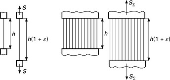
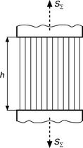
Applying the blending theory according to Hamburger (1949), the fibre bundle is regarded as a blend of two types of fibre (Fig. 7.30) and all fibres of one type have the same force-strain curve S = S(e), the same strength P and the same breaking strain a.
In the following discussion, the fibre of one type having a smaller value of the breaking strain is denoted as No. 1, the other type of fibres is denoted as No. 2. (These numbers are used as subscripts, see Table 7.8.) For fibre No. 1, we have


For fibre No. 2, we get in a similar way
The maximum forces in a bundle are shown in the stress–strain curves in Fig. 7.31. For the interval ε < a1 ⇒ max. at e = a1, which results in

For the interval ε ϵ (a1, a2) ⇒ max. at ϵ = a2, which results in
In the interval ε>a2⇒ all fibers are broken:
The strength of the fibre bundle can then be calculated with

where P1/t1 stands for the tenacity of fibre No. 1 (e.g. N/tex), P2/t2 stands for the tenacity of fibre No. 2 (e.g. N/tex) and S2(a1)/t2 is the specific stress of fibre No. 2 (e.g. N/tex) at ε = a1. The bundle tenacity PΣ/T is then given by
and the breaking strain of the bundle can be calculated with
Figure 7.32 shows a graphical representation of the resulting equation [7.158]:

7.32 Graphical representation of equation [7.158].
For the minimum bundle tenacity, there are two possibilities according to Fig. 7.32:


Now, the minimum bundle tenacity is the minimum of the three calculated values PΣ/T. It is important to note that after adding fibres with a higher tenacity, the tenacity of the resulting bundle can decrease! This theory can also be applied for a rough estimation of combination staple fibre yarns. In this case, it is necessary to use analogous values of the corresponding individual component yarns in place of the fibre parameters. In this case, P1/t1 then stands for the tenacity of the first single yarn (100% material No. 1) and P2/t2 for the tenacity of the second yarn (100% material No. 2). S2(a1)/t2 is the specific stress of the first yarn (100% material No. 2), when the strain is equal to its breaking strain, i.e. (ε = a1); all, e.g., in N/tex. A more detailed description of this model can be found in Neckář and Das (2006).
7.10 Examples of models of fibrous assemblies and yarns
In Keefe et al. (1992) and Keefe (1994), a mathematical model for fibrous assemblies is developed where yarns are regarded as three-dimensional structures. In the earlier model, the yarns are considered to be inextensible and incompressible whereas in the later model, this limitation is overcome. A rope-like structure can thus be described and analysed composed of a twisted bundle of individual yarns.
Ghoreishi et al. (2007a) describe a model for synthetic fibre ropes. They develop one model for an assembly of a large number of twisted components and another one for a structure with a straight core and six helical wires. This 1+6 model is then used to predict the axial stiffness of the rope and the correlation to measured values is good. The mechanical behaviour under tension and torsion is described in a subsequent paper (Ghoreishi et al., 2007b). The tension-torsion coupling behaviour of the constituents is used to deduce the behaviour of the rope. A comparison with measurements shows the validity of the model.
Carnaby and Postle (1991) discuss different mechanisms of fibre deformation and slippage which contribute to the stored elastic strain energy and work done against friction during the deformation of staple-fibre yarns. They assume continuity in the strain and energy fields and thus suggest using a unit cell of fibres in order to describe the mechanical behaviour of a yarn.
Liu et al. (2007) designed a model for wool yarns. It is based on discrete- fibre modelling principles, hence the yarn is considered as an assembly of a large number of discrete fibres. The movement of fibres during deformation and their final positions after deformation are determined by their need to minimize the tensile strain. The dependency of the yarn strain on fibre tension, bending and torsion is derived. A comparison with experimental data shows an acceptable accuracy of the predicted values.
An earlier model to predict the strength of yarns based on the fibre properties is described in Iwona (1992). The mechanisms of yarn failure depending on the interfibre friction is also analysed in Broughton et al. (1992). They found that even slight changes in the interfibre friction can lead to large changes in the yarn strength.
Phillips et al. (2010) investigated the mechanical governing equations that describe the torsional behaviour of multi-ply yarns under tension. They found that the slope or gradient of the torque due to tension (Fig. 7.8), the fibre number, moduli and diameter have the greatest influence on the torsional properties. The tensile properties of textured yarns are discussed in Kawabata and Sasai (1978). They apply a model where each fibre contributes independently to the yarn’s tensile property. Then, they model the tensile property of a crimped single fibre (helical coil). Applying this to determine the tensile property of a textured yarn shows a good correlation with measured values.
A comprehensive list of many more interesting papers on the subject of this chapter can be found in Neckář and Das (2012).
7.12 References
Braschler, E. Strength of cotton yarn. Moscow: Gizlegprom; 1939.
Broughton, R.M., El Mogahzy, Y., Hali, D.M. Mechanism of yarn failure. Textile Research Journal. 1992; 62(3):131–134.
Carnaby, G.A., Postle, R. Discrete fiber versus continuum models in the mechanics of staple yarns. Journal of Applied Polymer Science: Applied Polymer Symposium. 1991; 47:341–354.
Gegauff, C.M. Strength and elasticity of cotton threads. Bull. Soc. Industr. Mulhouse. 1907; 177:150.
Ghoreishi, S.R., Cartraud, P., Davies, P., Messager, T. Analytical modeling of synthetic fiber ropes subjected to axial loads. Part I: A new continuum model for multilayered fibrous structures. International Journal of Solids and Structures. 2007; 44(9):2924–2942.
Ghoreishi, S.R., Cartraud, P., Davies, P., Messager, T. Analytical modeling of synthetic fiber ropes subjected to axial loads. Part II: A linear elastic model for 1+6 fibrous structures. International Journal of Solids and Structures. 2007; 44(9):2943–2960.
Hamburger, W.J. The industrial application of the stress–strain relationship. Journal of the Textile Institute. 1949; 40:700–718.
Hearle, J.W.S., Grosberg, P., Backer, S. Structural Mechanics of Fibres. Cambridge: Yarns and Fabrics; 1969.
Iwona, F. New approach for predicting strength properties of yarn. Textile Research Journal. 1992; 62(6):340–348.
Kawabata, S., Sasai, T. Theoretical analysis of tensile properties of textured yarns. Journal of the Textile Machinery Society of Japan. 1978; 24(1):13–18.
Keefe, M., Edwards, D.C., Yang, J. Solid modeling of yarn and fiber assemblies. Journal of the Textile Institute. 1992; 83(2):185–196.
Keefe, M. Solid modeling applied to fibrous assemblies part I: twisted yarns. Journal of the Textile Institute. 1994; 85(3):338–349.
Liu, T., Choi, K.F., Li, Y. Mechanical modeling of singles yarn. Textile Research Journal. 2007; 77(3):123–130.
Malinowska, K. Evaluation of Shape Coarseness of Fibre Cross Sections. Przeglad WHokienniczy. 4, 1975.
Neckář, B. Yarns: Creation, structure, properties. SNTL Prague; 1990.
Neckář, B., Das, D. Mechanics of parallel fibre bundles. Fibres & Textiles in Eastern Europe. 2006; 14(3):23–28.
Neckář, B., Das, D. Theory of Structure and Mechanics of Fibrous Assemblies and Yarn. CRC Press; 2012.
Phillips, D.G., Tran, C.-D., Fraser, W.B., van der Heijden, G.H.M. Torsional properties of staple fibre plied yarns. Journal of the Textile Institute. 2010; 101(7):595–612.