
The finite element method (FEM) and its application to textile technology
Abstract:
This chapter describes the basics of the finite element method (FEM) and its application for modelling of textile structures. It gives a brief introduction to the basics of the modelling of mechanical systems in the static and dynamic cases, some of the ideas behind the finite element method and a short overview of FEM software.
6.1 Introduction
This chapter describes the basics of the finite element method (FEM). Since the development of the method and the publishing of the first book about it by Zienkiewicz and Cheung (1967), more than one hundred books have been published about the FEM, mostly written especially for engineers, mathematicians, programmers and ‘dummies’. The aim of this chapter is not to summarize the contents of these books or to cover all the aspects they cover but to give a brief introduction to FEM for textile engineers and students. They may have learned about the FEM in lectures on statics, but do not know how to use it in dynamics. Alternatively, they may have studied chemistry, fluid dynamics or physics, but not enough continuum mechanics. As a result they may need to model a textile structure with FEM software, with not much knowledge of what is hidden behind the windows and buttons. For experienced FEM users, there could be some interesting points mainly in the comparison of explicit/implicit method and in some of the applications at the end of this chapter.
Engineers and scientists in general often analyse objects and processes by creating simplified mathematical models. The goal is to understand these objects in order to be able to predict their characteristics and in the ideal case to be able to design objects with improved or special characteristics. Every material object has three geometrical dimensions (x1, x2, x3). The geometry and the properties of this object can be defined to be a function f(x1, x2, x3) of these three dimensions. The geometry and the investigated property can change during the timespan t. This function thus depends on four variables f(x1, x2, x3, t). Applying the laws of nature about mechanics, thermodynamics, acoustics, etc. to this property, a set of equations for the investigated object can be defined. They describe the dependencies between its variables and the object parameters p1, p2, etc.:
Normally, in equation [6.1], there are several terms consisting of the partial derivatives ∂f/∂x1, ∂f/∂x2 of f with respect to the independent variables x1, x2, e.g. the coordinates in the principal direction. Such equations are named partial differential equations (PDE) and they are used to describe problems in the statics and dynamics of elastic bodies, propagation of sound or heat or fluid flow, electrostatics and dynamics and a wide range of other phenomena. In general, it is not possible to find an exact analytical solution of the partial differential equations. The FEM is an numerical method for solving PDE, developed over the last 60 years, owing to the increasing computer power which is required for matrix calculations (Fig. 6.1).

6.1 Part with nonlinear geometry: (a) CAD view; (b) the same part meshed with regular finite elements; (c) deformed part with the simulated Von Mises stresses.
The idea of the FEM is that the investigated body is split (meshed) into a set of small parts, named elements with known finite size (finite elements) for which keypoints (nodes) the equations have an analytical solution (Fig. 6.1b). The nodes at the edges of one element are simultaneously nodes of some of the neighbour element. Because of this, the solutions of problems for both neighbour elements have to have the same values at these nodes. In order to ensure this, a system of equations for all the nodes is solved. Due to the linear elastic bodies, this system of equations is linear and can thus be solved within a very short period of time using a computer and, thus, a solution for a complex geometry can be found quickly. A big advantage of today’s FEM software for engineers is that all the numerical methods for the solution of the PDF for each element and for solving the whole linear system remain hidden from the user. The user has to prepare the geometry, the material, constraints and loads for the system and then the software more or less automatically looks for a viable solution. Because of this, this method is very popular, especially for applications where a stable automatic solution can be defined.
6.2 Modelling of mechanical systems
The modelling process of mechanical systems consists of several steps (Fig. 6.2). The real system has to be idealized into a physical model, then a mathematical model is created and solved. This section discusses important issues of this modelling process in general.

6.2.1 The modelling process
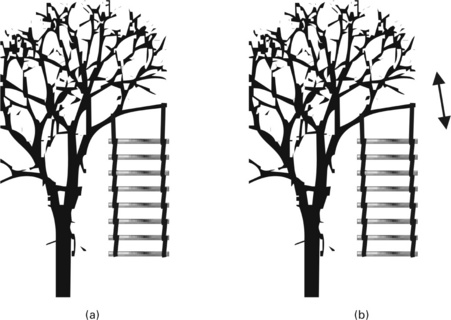
During the modelling with FEM, the real system (Fig. 6.3a), like a tree with a ladder, has to be idealized first in order to achieve a somewhat simplified physical system. This first step is the building of the physical model, where certain assumptions have to be made. For example, it could be assumed that all steps consist of the same material, they have the same geometry and mechanical properties, and that the connections between them are the same. This idealization step generates the first source for errors, e.g. influences from the differences of the weight and the geometry of the steps are already excluded and will not be considered in the next step. The created physical model (Fig. 6.3b) represents the investigated system in a simplified way, so that some analytical or numerical method could be applied. During the FEM modelling, a discrete model of the system has to be created (Fig. 6.3c), which consists of beams and ropes, connected at the nodes. The chosen discretization method leads to a discretization error, e.g. using one beam element per step, so only a coarse approximation of the step deformation can be achieved, and the real deformation cannot be represented.

6.3 The way between the physical object and FEM model: (a) real object − ladder on a tree; (b) physical model − consists of equal steps; (c) discretized model − the steps are represented as a beams and ropes, connected at the nodes.
Having defined the elements and the nodes, as well as the problem type which has to be solved (static, dynamic, vibration, etc.), the equations for this system can be created and solved. These equations represent the mathematical model of the system. The advantage of using commercial or non-commercial, but well-tested and evaluated, FEM software is that at this step, the methods are well investigated and the risk of an additional error is minimized. In most standard load cases with standard elements, an error can be ruled out. This is not the case for the solution of the mathematical model, where the user still has the possibility to influence the step size during the integration, etc., so numerical errors are possible. In the case of FEM in mechanics, the calculated solution represents the displacements of the nodes. This is a solution of the discrete system and it differs from the real system − because of all previously described error sources. If the difference between this solution and the real situation of the system is less than the allowed error, it can be assumed that the modelling was successful and the model is verified.
6.2.2 Types of problem from the mechanical point of view
The aim of the FEM in statics and dynamics is to calculate the behaviour of mechanical bodies and systems. In the different subareas of classical mechanics, the objectives of the FEM differ. The equation of the dynamics equilibrium of an elastic body consists of different components:
The first component, K ⋅ u, describes the internal elastic forces of the body, which are proportional to its stiffness (matrix) K and the displacement vector u. The second element, ![]() , describes internal viscous forces, which are proportional to the velocity of the nodes. These forces are important for polymer materials or can be used to describe air resistance. The third component,
, describes internal viscous forces, which are proportional to the velocity of the nodes. These forces are important for polymer materials or can be used to describe air resistance. The third component, ![]() , represents the forces of inertia, which depend on the acceleration of the system and on its mass M. All external forces are represented by the vector on the right-hand side of the system − F. The solution of the system [6.2] represents the motion of the steps (Fig. 6.4) and their deformation due to the given loads.
, represents the forces of inertia, which depend on the acceleration of the system and on its mass M. All external forces are represented by the vector on the right-hand side of the system − F. The solution of the system [6.2] represents the motion of the steps (Fig. 6.4) and their deformation due to the given loads.

If the deformations inside the steps are negligible compared with the displacements (to the motion), then the internal forces and the damping can be neglected and it is possible to reduce the system to:
The motion law can be derived by equation [6.3]. For the investigation of the vibrations of the body, the natural frequencies and forms have to be found. If the motion of the system with consideration of the elastic changes in the body has to be found, the system [6.2] has to be completely solved, with the right-hand side set equal to zero:
These natural frequencies and forms then represent then the vibrations of the steps, if the branch is not moving (Fig. 6.5a). If the branch is swinging with a frequency ɷ, then the forced vibration of the system can be investigated by integrating equation [6.5]:
6.5 Frequencies: (a) the independent motion of the ladder; (b) forced vibration − the behaviour of the ladder if the branch of the tree is moving or vibrating.
All these cases consider the dynamics or the transient processes of the system. At present, the dynamic equations are solved usually, but not in all cases, using explicit numerical methods, where the displacements at the later time state are calculated using the state of the system at the present time. With implicit methods, the state of the system involving both the current and the subsequent state is calculated. They are usually used for static problems (Fig. 6.6). In statics there is no velocity and acceleration of the body and equation [6.5] becomes the simple form for linear (or nonlinear) systems:

6.6 Static calculation − the ladder and its components are not moving; their deformations and the forces at static equilibrium are investigated: (a) initial state; (b) deformed state.
In this case, the stiffness matrix K and the forces F are known at the current time step and the nodal displacements have to be found solving the system [6.6]. For this case, different discretizations are also possible, e.g. the steps, assuming a constant cross-section, can be represented by a single beam (Fig. 6.7b). A meshing of the steps with smaller elements requires more computational time, but allows a more precise solution and can be used even if the steps have a more complex geometry, which cannot be simply represented by a beam.
6.2.3 Elasticity theory for FEM calculations
For FEM calculations, three laws are required for the modelling of mechanical systems − kinematic, constitutive (material) and equilibrium.
Kinematic
The kinematic equations represent the relation between the nodal displacements and the internal deformations (strains) of the mechanical system. Figures 6.8 and 6.9 explain the fundamentals of the kinematic relations based on a square figure ABCD. Figure 6.8a shows a plate ABCD with an infinitessimal side dx. The mesh inside the figure is shown only to visualize the deformations inside the plate. When point A moves inside the XY plane, its displacement is given by

6.8 Kinematic relations during small deformations of elastic body: (a) initial state; (b) pure elongations without change of the angle between the sides (c) shear deformation.

The side AB, having an initial length dx will become longer (or shorter) with
Thus, the new length A*B* is given by
The linear elongation in X direction is the change of the length related to the initial length, so that:
In the three-dimensional case, the linear elongations in the three main directions can be derived as follows:
In addition to the linear elongations, the body can be deformed so that the angles of it change. In the case of the analysed plate ABCD (Fig. 6.8c), the angle ∠ BAD can change. This depends on the rotations of both sides AB and AD and can be represented as a sum of the angles φ1 and φ2.
It could be proven (for instance in Rieg and Hackenschmidt, 2003), that
and the change of the angle ∠ BAD in dimensionless form is
The variable γxy is called the engineering shear strain. According to the definition, we have:
Then, the entire strain matrix becomes a tensor


Equations [6.11] and [6.16] represent the connection between the displacements of the nodes and the strain in the body in the linear case (small deformations) and build the kinematic equations. For larger displacements, the accuracy of these equations is not sufficient, since they are derived using only the first term of the Tailor development of the relation uB = f(uA, dx). In such cases, more terms in the development have to be used or other equations for the relations between displacement and strain have to be derived. Since the nonlinearity in these equations is based on pure geometrical relations, the problems are known as ‘problems with geometric nonlinearities’. For these, special options in the FEM software have to be activated to ensure that the proper equations are used. More details about geometrical nonlinearities are given in Section 6.5.
Constitutive equations
Constitutive equations represent the relations between the deformations of the system and the internal stresses. These are usually named material law, because they represent the behaviour of the material of the modelled object. In the simple case of a linear elastic material (e.g. a spring), the constitutive law is Hooke’s law, here represented in a matrix form:
where the stresses in vector form are given by
The normal stresses result from tension or pressure applied on the working plane, for instance σxx (Fig. 6.10). The tangential τxy stresses are caused by shear forces. The first symbol shows the plane index, where the stresses are applied and the second symbol the direction of the forces. For example shear stress τxy is applied in the plane x, perpendicular to the x axis, and its direction is parallel to the y axis.

The strains here are in vector form:
and the elasticity matrix is then given by

consisting, in the general case, of 21 independent constants, representing the material properties presented as a relation between stress in one direction and strain in the same or another direction.
The elasticity matrix is symmetrical, because coefficients with the same digits are equal, e.g. c21 = c12. For most engineering materials, such as metals, this matrix is filled only by two independent constants − the elasticity modulus E and the Poisson ratio v:
In some special cases, where the Poisson ratio is equal to 0.5, the volume of the body does not change during deformation. In this case of incompressibility, nonlinear material models have to be used. Some more information about linear and nonlinear models is presented in Section 6.7. If the relation between the stresses in the body and its deformation is nonlinear, then we have
This model is labelled ‘model with material nonlinearity’. Such problems require the use of special numerical methods as standard models would fail.
Equilibrium equations
The equilibrium equation describes the static or dynamic equilibrium of all internal and external forces of the system. In the static case, the equilibrium equation is
where K is the stiffness matrix of the system, u is the vector with the nodal displacements and F represents the external forces (Fig. 6.11). In the dynamic case, suitable equations from Section 6.2.2 are used instead of equation [6.23]. The left-hand side of equation [6.23] represents the internal forces, calculated on the basis of the displacements of the single nodes and the stiffness of all the elements. How the stiffness matrix K aggregates kinematic relations equations [6.11] and [6.16] with the constitutive equation [6.21] in one matrix is described in the next section.

6.2.4 Static equilibrium and element stiffness matrix
One of the ideas of the FEM is that the displacements at every point inside of one finite element U(x, y) = [u(x, y) v(x, y)]T can be represented by interpolation of the nodal displacements ui using the known function Ni(x, y)
The functions Ni (x, y) are named shape functions. They can be linear, quadratic or from a higher power which determines the order of the element. If the functions are linear, the element is of first order, if quadratic-second order and so on (Fig. 6.12).
6.12 The displacement of any point inside the finite element is presented as a function of the nodal displacements.
Some examples of shape functions are given in the next section, where the different elements are described. Since the shape functions are given and selected during the development of the FEM code and not during the modelling, the main operations, like differentiation over these can be performed analytically. This minimizes the numerical errors from numerical differentiations, and simplifies and speeds up computations. The strains εij (here, only the strains for the two-dimensional case are taken) can be presented using a differential operator L and a displacement vector U as follows:
Using the shape function for the displacements, these become
which, in matrix form, with the displacements of the nodes leads to: U(i)
Hence, the strains from equation [6.25] become
where the matrix B consists of the differentiated form functions. The relations for elements with other numbers of nodes in 2D and 3D space are similar.
At that point, the principle of the virtual displacements will be applied. If the system deforms with a virtual displacements δε the virtual internal work δWi and the external work δWe have to be equal:
The virtual external work is due to the external forces and can be represented by
where P stands for the distributed volume forces and F(i) represents the concentrated nodal forces.
The virtual internal work δWi can be derived as the increase of the internal (potential) energy, or as a product of the displacements and the stresses (work is equal to the product of way δεT and the force) according to: σ ⋅ dV
The equilibrium of the internal and external work is then:
Taking into account equations [6.28] and [6.27], we get:
Applying the rules for matrix transpose (AB)T = BTAT that leads to
The displacements δU(i) are not dependent on the volume and the equilibrium between the internal and external forces has to be true at every displacement, so we have:
According to equation [6.17], the stresses σ = C ⋅ ε are dependent on the material law and the strains on the displacements according to equation [6.28], hence: BU(i)
If the nodal forces on the right-hand side are not considered for simplification, then we get:
Considering the element stiffness matrix as
the main equation of the FEM for the static problems in local, element coordinates is derived as:
In this equation, the displacements, the forces and the stiffness matrix are in the element (local) coordinate system. For the solution of the entire system of elements in one body, these have to be transformed to the global coordinate system.
It is important to note in this case that:
• equation [6.39] is linear and can be solved according to the unknown displacements using standard libraries and methods;
• the stiffness matrix is constant (for linear cases) and can be calculated on the basis of simple matrix operations using the form functions. These are defined before solving the problem and their differentiation can be done analytically, so that the matrix B is known during the building of the mathematical model at the moment and the appropriate element is selected.
The different element types are discussed in Section 6.3, and the main steps of the performing FEM simulation with available FEM software are explained in the next section.
6.2.5 Dynamic equilibrium − explicit versus implicit integration
In the same way as in the previous section, equation [6.39] can be derived in the case of additional forces from the acceleration and damping in the form (with global coordinates and the subscript (i) for the displacements is skipped for simplification):
where M, C and K are the mass, damping and stiffness matrices of the entire system, U is the displacements vector of all nodes, and F is the force vector with all acting forces in global coordinates. This equation consists of first and second order derivatives of the displacements and can be solved during implicit or explicit integration. The displacements U, velocities U and acceleration Ü have to be calculated at every time step tn. To solve it, the equation has to be transformed into an algorithm-dependent time-difference equation by quantizing and replacing
with some finite difference such as forward differences
In the explicit integration, the equation for accelerations is written in the same (analogous) way through the actual, known displacements.
The displacements Un, velocities ![]() , accelerations Ün and the forces Fn have to be calculated at every time step tn. Actually, in order to calculate the accelerations and the velocities with some of the finite differences during the time tn, the displacements and the next and/or previous time step must be known, depending on the type of the used finite differences. The problem is that the displacements in the next time step (in the future) are not known. At that point, depending on the method for the solution of this problem, two approaches can be used, which lead to two different groups of the FEM and software − explicit FEM and implicit FEM (Fig. 6.13).
, accelerations Ün and the forces Fn have to be calculated at every time step tn. Actually, in order to calculate the accelerations and the velocities with some of the finite differences during the time tn, the displacements and the next and/or previous time step must be known, depending on the type of the used finite differences. The problem is that the displacements in the next time step (in the future) are not known. At that point, depending on the method for the solution of this problem, two approaches can be used, which lead to two different groups of the FEM and software − explicit FEM and implicit FEM (Fig. 6.13).
![]()
6.13 The ideas of the explicit (a) and implicit (b) integration of the differential equation. For the explicit integration the next time point is calculated based on the information from the previous time point (a). During the implicit integration, a system of the unknown variables have to be solved at each time step, in order the proper solution for the next time point to be found (b).
For explicit integration, the next time point is calculated based on the information from the previous time point (a). During the implicit integration, a system of the unknown variables has to be solved at each time step, in order to find the proper solution for the next time point (b).
During explicit integration (Fig. 6.13a), the displacements at the next time step are calculated using the displacements of the previous time step and the velocity. This procedure is stable only for time steps smaller than a critical limit and can be applied only for some of the methods for the calculation of the velocity (for instance central differences). For instance, if the damping in equation [6.40] is neglected, for the time step tn, we get
and the new point is extrapolated for the next time step n + 1.
Assuming that the displacement can be interpolated as a linear function of time, the velocity at one step after the current one is given by:
The acceleration at the current time step can then be calculated as:
where replacing [6.45]
The next displacement can be written as:
Since the accelerations depend on the forces
the new point can be calculated as
Only the information about displacements and the forces (here, the space derivatives of the partial differential equations are hidden) from the previous time steps is used. In contrast, during implicit integration, the displacement at the new time point is unknown but it has to be found so that the forces during the new time step satisfy the equilibrium equation as well [6.44]
where the acceleration Ün+1 is calculated analogously to equation [6.48].
After transformations and some assumptions (linear acceleration) the equation can be written in the form
Here the coefficients ai depends on the time step and the chosen integration method (central differences, Newmark, Fox-Goodwin) and the effective stiffness and force matrices are named Keff and Feff,n+1, respectively. As equation [6.53] shows during the implicit integration a special system of linear equations has to be solved at each time step. For this, the inverse matrix of Keff has to be found, which is a computational-intensive operation and not in all cases solvable. For large deformations, this matrix depends as well from the displacements, and then system [6.53] becomes nonlinear. From other point of view, if the numerical method is chosen properly, for instance Newmark, it is unconditionally stable, independent of the time step and can work with large but cost intensive time steps.
For the explicit integration only the inverse matrix of the mass matrix

has to be calculated, and this is a trivial operation as

The mass normally remains constant and its inverted matrix can be calculated once at the beginning of the integration process. However, for implicit integration, the inverse of the stiffness matrix has to be calculated at every time step. For nonlinear problems, the stiffness matrix depends on the displacements and thus several iterations have to be done until the displacement vector and the stiffness at the new time step are found.
Generally, because of the very small time step required, the explicit integration is used for simulations where very short timescales or nonlinear processes have to be analysed. These are for instance the crash (and generally the contact) simulations. Because the calculations can be done in parallel, the amount of steps is no longer a problem for the calculations. In all other nearly linear cases, the implicit integration offers a fast solution with large time steps. These and other differences between implicit and explicit method of the integration of the equilibrium equations are summarized in Table 6.1 (ESI Group, 2011).


6.2.6 Structure of typical FEM software
FEM calculation requires several steps and for most of these, separate programs (tools) were developed (Fig. 6.14). The preparation of the FEM model is done by the preprocessor. If the problem type (static, dynamic) is specified at the beginning, some of the software packages automatically select the elements and materials which are suitable for this kind of analysis, which reduces the risk of errors. The information about the material or geometric nonlinearities or other special properties of the modelled object has to be specified as well, in order for the proper solver type to be chosen.
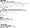
The geometry of the modelled system has to be built inside the preprocessor or imported from CAD. In the case of FEM calculations of machinery, which are designed in CAD software, it is suitable to use the direct import of the geometry data. In other cases, e.g. complex textile structures, it is better to build their geometry inside the preprocessor or with special programs. For each task, enough material properties have to be specified − depending on the problem only the elasticity modulus and Poisson ratio are sufficient in case of a linear static analysis of isotropic material, but to take into account also dynamic forces, the density is required too.
The selection of the element types is the most important step. Usually, several elements from similar types are available, but these have different options which in turn define different degrees of freedom.
With all these data, each body has to be discretized into small elements from the selected type: the meshing process. In some cases, the meshing procedures create nodes very close to each other. They then have to be merged and the mesh has to be checked. Finally, the boundary conditions and the loads have to be defined. For static problems, the body has to be statically determined or over-determined. All this information is usually stored as a file and sent to the solver, which solves all the equations and writes the results (unknown displacements and other parameters) into a file again. The analysis and the visualization of the result requires separate software, known as the postprocessor, which is able to read the displacements of the nodes, to recalculate the forces within the elements and to display these in the proper places.
6.3 Elements of elastic models
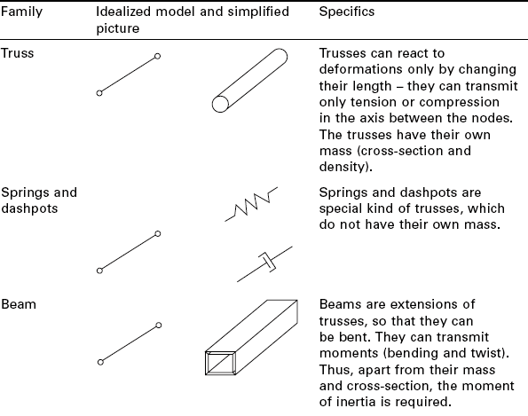
The objects can be presented during modelling using different families of finite elements, presented in Table 6.2. In addition to the family type of the element, its behaviour is determined by its dimensionality, number of nodes and number and type of the degrees of freedom. The beams and trusses can exist as 2D or 3D elements. The 3D beams and trusses can move and deform only in one plane, for instance x–y, which reduces the size of the matrices and the calculations in comparison to the use of the 3D elements. The number of the nodes is at least equal to the number of the element corners, but the elements from higher order have nodes also between the corners. Elements that have modes only at their corners use linear interpolation in each direction. They are called linear elements or first order elements (Fig. 6.15a). Elements with midside nodes use square (or higher order) interpolation and are called second (or higher) order elements (Fig. 6.15b). Every node can have different numbers and types of degrees of freedom at the node from zero up to three translations and from zero up to three rotations. For instance the node of one-dimensional truss element has only one degree of freedom − the translational displacement in the x-direction.
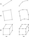
6.15 Elements with different order: (a) first order elements and (b) second order elements with midside nodes.
6.3.1 Trusses and beams
Truss elements are used for structures, which can transfer loads only in one direction − the truss axis. They can work at tension and/or pressure and are defined by two nodes − both of the ends of the truss. Depending on the problem, two or three degrees of freedom per node can be available: for the plane problems only two translations per node are required, while for 3D problems all three translations have to be considered (Fig. 6.16). It is assumed that the truss element is a straight bar with a uniform crosssection. The displacements between the nodes are calculated using the shape functions (Fig. 6.17).

Depending on the displacements of the both ends, here called v1 and v2, the displacement in the one direction of any point of the truss element can be calculated using:
where x is the local coordinate, and L the length of the element. It is simple to demonstrate the strain calculation using analytical differentiation of the shape function
After that the entire element stiffness matrix K according to equation [6.38] can be calculated. The advantage of using truss elements with two nodes lies in its simplicity and shorter calculation time, but the disadvantage is in the only linear approximation of the displacements within the element. However in such an element, the loads can be applied only at both nodes at the edges. In the cases where loads have to be applied arbitrarily along the axial direction of the truss, use of higher element order trusses is more suitable. The simplest one is of second order and has a midpoint node (Fig. 6.18).

The shape function matrix for this case, depending on the coordinate ξ will be
since x starts from zero up to the element length L, and the shape function has to have value 1 at the nodes, a change of the independent variable from ξ to x using
is required and after that the differentiation about x has to be done in order the matrix B and the end the element stiffness matrix to be calculated. This operation remains hidden for the normal user of FEM software, but an understanding about the shape functions and the proper choose of element is important for the proper modelling.
Trusses are useful for the presentation of frame, yarn and rope structures, where these are working under tension without being bent. For instance, the ropes in a paraglider can be modelled by trusses (Fig. 6.19). Because of the computational and algorithmically simplicity, trusses are used very often to model different textile structures as a net shape structure. Figure 6.20 shows a model of a weft knitted structure as a hexagonal net by de Araujo et al. (2004) and draped structure. Figure 6.21 shows similar application for spacer warp knitted structures (Kyosev and Renkens, 2010a). Interesting application of trusses for the modelling of textile structures can be found as well in Cherif (1998).

6.19 Principal stress in paragliders, simulated with CalculiX. With kind permission of Thomas Ripplinger, ADVANCE Thun AG, Thun, Switzerland.

6.20 Modelling of plain weft knitted structures with trusses: (a) yarn axes of the weft knitted structures; (b) FEM model, using the yarn contact places as nodes; (c) simulated draped weft knitted structure over ball, according to de Araujo et al. (2004).

6.21 Application of truss elements for mechanical adjustment of warp knitted structure: (a) idealized tricot structure in pure geometrical model; (b) yarn axes and positions of the nodes for the modelling;
Beams are extensions of trusses. They can transfer bending moments at the nodes as well. Thus, at the nodes, in addition to the displacements, a rotation in the beam plane for 2D beams and three rotations for 3D beams are added as degrees of freedom to each of the nodes. Thus, the 3D beam (if implemented in the software and if this option is chosen) can additionally carry twist moments due to the rotation of the cross-section (Fig. 6.22). Beam elements are used for creating models where the deformation of the beam and its bending rigidity have to be considered. The beam models differ in how their cross-section follows the deformations of the axis − and because of this in the libraries of the FEM software, different beams are available. One popular element is the Hughes-Liu beam element (Hughes, 1981), in which the rigid body rotations do not generate strains (is incrementally objective). This model is computationally efficient and compatible with brick elements and includes finite transversal shear strains. The Belytschko beam (Belytschko et al., 1977), has the capability to allow large rotations. Figure 6.23 shows successful modelling of woven structure on a filament basis (Durville, 2010), where each filament is modelled as a beam (but presented on the picture as a solid body).

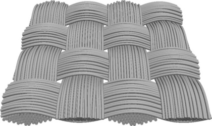
6.23 Plane weave structure, where the filaments of the yarns are modeled with beam elements. Courtesy of Damien Durvile (Durville, 2010).
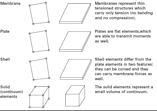
6.3.2 Membranes, plates and shells
Membranes, plates and shells are elements that have been developed for the presentation of thin flat structures, so that their behaviour is correctly represented without explicit presentation of the thickness of the structure. For this reason, they are suitable for structures where the thickness is negligible related to the other dimensions of the structure. Typical examples are textiles, foils, plates, etc. The thickness of the structure has to be defined as a parameter and it is used in the calculations.
The membrane elements are the plane analogue of the trusses as a onedimensional element. The nodes of the membrane elements have only translations as degrees of freedom and they can transmit only stresses which are in their plane, but no bending loads (Fig. 6.24a). These elements can be curved as well. Figure 6.19 presents a simulation of a paraglider within the software CalculiX, where the main structure is presented by membrane elements. Another typical case is the building roofs under tension, such as stadium roofs (shown in Fig. 6.25).
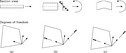
6.24 Membranes, plates and shells in a section view and degrees of freedom: (a) membrane element; (b) plate element; (c) shell element.

6.25 Membranes − Olympic stadium in Munich (Tobi87, 2007).
The plate elements can be considered as a 2D extension to the beam elements: they are able to transmit bending moments (no in-plane torsion) andcan model structures, which stress distribution through the thickness is linear. Important is, that the plates have to remain planar after the deformation.
For the more complex cases of combinations of the loads between membrane and plate load, the shell elements have to be used. There are several definitions of shell elements (also of plate elements, depending on their thickness) and careful studying of the programmed behaviour of the shell elements is required before choosing the proper one for a certain model. The main differences between these elements are presented in Table 6.3. All the elements can be implemented and used usually as three or four node elements from first order or as six or eight node elements of second order. The second order elements can lead to stable results even within a coarse mesh, whereas the first order elements require a finer mesh to achieve the same stability.

Elements for axisymmetric case
There are several situations of the simulation of rotational symmetric bodies like spindles, spinning rotors, carding rollers, etc. for which the calculations and the computational time can be significantly reduced if rotational symmetry is being used. In such cases, different axis-symmetric elements are used, which differ in their definitions depending on whether only the geometry is axisymmetric or the geometry and the loading are both axisymmetric.
6.3.3 Solid elements
In the general case where the solid body has to be modelled as a solid without any restrictions and simplifications, solid (3D or ‘volume’) elements are used. In this case, several effects can be recognized and modelled properly, which cannot be seen during the modelling with beams or 2D elements because of their simplified definition. In several cases, especially with textiles, it is harder to prepare the geometry and the mesh for solid elements. It is harder to check for errors, because several places remain hidden and only with special calculations of well-defined meshes, quality criteria can be recognized. In addition, solid elements require much greater computer resources, e.g. a much greater computing time. Despite these disadvantages, the use of solid elements allows a more complex and full instigation of the deformations and they are therefore widely used.
Figure 6.26 shows four basic types of solid elements − the four node tetrahedron element and the eight node brick element ((a) and (c)), as well as their second order versions with nodes at the middles of the element edges. An example of a ring spinning spindle, its mesh and the calculated von Mises stresses using solid elements are presented in Fig. 6.27. Figure 6.28 presents a deformed monofilament under bending, modelled with solid elements, after implicit FEM calculations and Fig. 6.29 depicts an example of a deformed plain weft knitted structure, where the yarns are meshed as well with solid elements.
![]()
6.26 Basic types of solid elements: (a) and (b) first and second order tetrahedron element, (c) and (d) first and second order (8 and 20 node-) brick elements.

6.27 Ring spinning spindle (a); meshed (b) and its stress distribution (c) (von Mises stresses) (Kyosev, 2002).


6.29 FEM model of a plain weft knitted structure: (a) front view; (b) side view; and (c) deformed state after explicit deformation with Ansys/LS-Dyna (Kyosev, 2006).
The modelling of the yarns with solid elements, as presented in Figs 6.28 and 6.29 is performed under the assumption of linear isotropic material behaviour. In fact, the yarns, especially staple yarns and multifilaments with less twist, have completely different behaviour in lateral directions than in the axial direction and to ensure proper modelling an anisotropic material model, which also considers shear stresses in the cross-section, must be used. The other challenge during the preprocessing of yarn structures is the setting of the proper material axis orientation − at each element, the orientation of the material has to be defined properly as well (Boisse et al., 2005).
6.3.4 Special elements for multilayer structures and composites
With the development and extended application of textile reinforced structures, FEM researchers and software developers started including special elements for such materials. In these elements, multiple layers of fibres with arbitrary directions can be defined. Examples of special shell elements for the draping simulation of woven composites are reported, for example, in the works of Philippe Boisse and his group, e.g. Hamila and Boisse (2008) and Hamila et al. (n.d.).
6.3.5 Contact elements
During the simulation of structures, where some parts are in contact with other parts or with themselves, special contact elements are required. These elements define:
• which elements or groups of elements have to be analysed, if contact occurs;
• what kind of reaction happens, if the contact is active, for instance if a penalty function has to be defined;
• how the contact time is calculated;
• whether the contact with or without friction has to be computed.
According to the first question, the contact elements can be classified into some general groups: contact between two solids, between two surfaces, between two beams or trusses, between solid/surface/beam and node.
The first group is used mainly in the CAD programs, where the solid bodies are well defined. The contact between solid bodies can be detected with very efficient computational procedures, but finally it has to be converted to contact between two surfaces. If the surfaces, which could start contacting, are known prior to the simulation, it is effective to define surface to surface (or beam to beam) contact elements only between these surfaces.
In other cases, large contact search procedures have to be started, which extend the computational time. Once detected and activated, the contact element has to generate contact forces at its nodes. The direction of these forces is usually in the contact normal and the value of the forces depends on the kind of the contact − elastic or rigid. The loops in Fig. 6.29 are calculated with surface-to-surface contact. All simulations of the textile processes like weaving and braiding require well-defined contact elements between the yarns and in the case of knitting additionally contact of the yarn with itself has to be checked. In cloth simulation, in addition to the calculation of the contact between body and the cloth, self-contact has to be considered. Examples of such simulations can be found in Schneider (2000) or Pickett et al. (2009) for the braiding process, and also in the several other works for weaving, knitting or braiding using LS-Dyna or Pam-Crash software.
6.3.6 Other elements
In several cases, efficient models can be built if some of the parts of the structures or the systems are not completely modelled, but only their behaviour is represented. For instance, during the modelling of the deformation of a warp yarn during weaving, it is not necessary to model the entire backrest system. If only the motion of the backrest is important, it can be represented in a model as a rigid body with a mass, connected with a spring and damper. For such cases, mass elements with one node and weight can be used for the modelling and the additional mass, or spring and damper elements with only two nodes and parameters (spring or damping constant) can be used for the calculation of the elastic forces.
6.4 Error estimation and refinement
6.4.1 Error estimation
After one model is created and calculated, it has to be proved. The most simple check of the numerical errors during the calculations is to refine the FE mesh by reducing the element size by half and to compare both solutions. The relative error for the deformations can be calculated for one node as:
where εL and σL are the displacement or the stress, calculated at one node, if the element size was L and σL/2 and σL/2 are displacement and stress, calculated using elements with the element size L/2. Usual errors reported in Reul (2010) assess the deformations to be between 5 and 20%, and for the stresses to be between 10 and 50%. If the accuracy of the calculations is not sufficient, usually the mesh has to be changed. In some cases, some nodes have to be moved, in order to avoid some singularities. The general cases for the refinements of the FE mesh are described in the following section, since most of them can be performed automatically with the software.
6.4.2 Refinement
Once a insufficient accuracy of the FE calculation is detected, the mesh has to be refined. Some of the FE packages perform this automatically, adapting the mesh in order to get a better solution. Using the h-method, the mesh is refined, so that the elements of the entire model are re-meshed with elements half their original size. In contrast, by using the p-method, the element size remains unchanged, but the order of the elements is increased. The combinations of these two strategies is known as the hp-method.
6.4.3 Some modelling errors
A lot of errors can occur during FEM modelling, some of which were described in Section 6.2.1. Here, only some errors are mentioned, which are connected to the meshing of the structures and the type of the solvers.
Proper problem/solver type
A major disappointment for textile researchers when they started using FEM for the simulation of textile structures was that as beginners they often started with some easy-to-use linear solver, so that the program ‘ crashed’, giving no answer or politely explaining ‘Calculations interrupted. The displacements are too large’. Since the textiles are very flexible structures, the deformations are large and the linear solvers for small displacements cannot perform the calculations stably. So, special attention has to be given of the choice of the type of the problem and the type of the solver.
Proper element type
The next common error is the improper selection of the element type. Modern software has built in several hundreds of element types but only a small number of these can represent the behaviour of the current structure properly.
Proper mesh size
More fine meshes in the areas with nonlinear geometry and with higher changes of the loads and more course meshes in the areas where less happens can limit the errors without significantly increasing computation time.
Avoid concentrated loads
The concentrated loads are used in the simplified mechanical calculations for beams and truss structures, but are not suitable for FEM analysis with plain and solid elements. One concentrated force is actually never applied on a single point; it is applied on a small surface. The same effect happens if beam or truss elements are connected with shell or solid elements − since the reaction of the 1D element acts as a concentrated load.
6.5 Nonlinear problems
As mentioned in Section 6.2, there are two places where nonlinearities can appear − if the displacements are not small, then the kinematic relations [6.11] and [6.16] will be no more valid and have to be replaced by other, nonlinear relations. In this case, the nonlinearity is geometric, because it is caused by pure geometric/kinematic relation. If the material law, expressed with the stress-stain equation is no longer linear, then the nonlinearity is caused by the material.
6.5.1 Geometric nonlinearities
The kinematic relations between the displacements of the points of one body (nodes) and its strains (equations [6.11] and [6.16]) are linear only in the case of small displacements. If the displacements become larger, the proper relations become nonlinear and the problem is classified to be ‘with geometric nonlinearities’. For such models, different numerical methods have to be applied. The geometric nonlinearities can be classified into several groups, as presented in Fig. 6.30.
The large displacements can cause small deformations in the body if the body can rotate (Fig. 6.31). This is the case for large rotations (Fig. 6.31c). If a part of the body is fixed, then the large displacements will cause large strain as well (Fig. 6.31b). The stress stiffening (or weakening) is another case of a geometric nonlinearity, where the structure is stiffening due to its stress state. Such effects are common for thin structures when their bending stiffness is very small compared with their axial stiffness. Typical examples are cables, thin beams and shells, where the stiffening couples the in-plane displacements with the transverse one. In the case of pure stress stiffening, the strain and rotations are small. Another geometric nonlinearity with small strain and small rotation is the spin softening, which occurs for a spinning (rotating) body. The vibration of this body can cause relative circumferential motions, which change the direction of the centrifugal load. The centrifugal load then tends to destabilize the structure (ANSYS Inc., 2011).

6.31 Examples for small displacements and for some geometric nonlinearities: (a) linear case with small displacements and small deformations; (b) large deformations; (c) small deformations but large rotations.
For all these geometric nonlinearities, different mathematical relations between displacements and strains have to be chosen. For the users of FEM software, this means that the available options have to be carefully selected, otherwise, the mathematical model will not represent the real situation and the resulting errors can become significant. Figure 6.32 presents the Screenshot of the Ansys® menu, where the analysis option with large displacements in Ansys® can be chosen. All these effects can be considered almost independent of the used material, because they are connected with the kinematic relations between the displacements of the points and the body deformations, which are in turn normally not connected to the material properties.

6.5.2 Material laws and nonlinearities
Models for elastic materials, where Hooke’s law between the strains and stresses is valid (equation [6.17]), are linear if there is no geometrical nonlinearity. For these models, also different material models are available, depending on the material constants from the material directions (Lekhnitskii, 1963). For isotropic materials, the properties of the materials are equal in all directions and only the elasticity modulus and Poisson ratio are required as described in Section 6.2. The Poisson ratio v describes the ratio between transversal and axial strain, if the material is stretched or compressed according to
The Poisson ratio has to be between − 1 and 0.5. For most materials, this value is between 0 and 0.5. Most metals have a Poisson ratio of 0.3. There are some materials such as cork, for which v = 0. There are some materials (mainly structures) which have a negative Poisson ratio − they increase their thickness when stretched. For isotropic materials, the shear modulus is calculated from the elasticity modulus and the Poisson ratio according to:
Orthotropic materials
Textiles and textile-based structures often have different properties in the directions where the main yarns are located − they are orthotropic (Fig. 6.33). The material properties in this case depend on the space directions, named here 1, 2 and 3 instead of x, y and z and there are nine constants, which have to be defined independently (E1, E2, E3, G23, G31, G21, ν23, ν13, ν12), three elasticity moduli, three shear moduli and three Poisson ratios. The stress–strain relation for orthotropic materials is simpler in its transposed form and is given by:

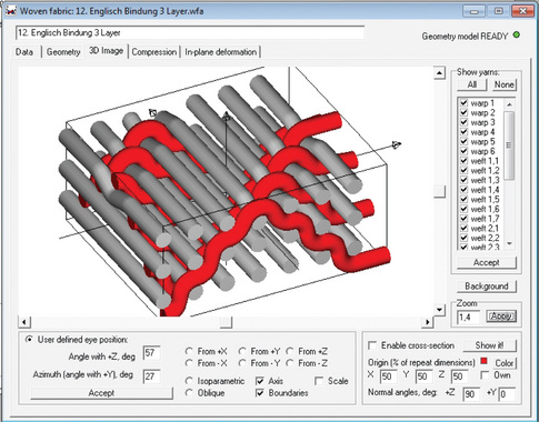
6.33 Woven structure as an example for an orthotropic structure: (a) the woven fabrics with main space directions (loading in these directions does not lead to shear); (b) loading different to the main directions for shear stresses; (c) deformed structure under the load in case (b).

Here, the directions 1, 2 and 3 have to coincide with the space directions of the material. In these directions, different from the three main directions, the material is anisotropic − shear and tension are applied. From the stiffness matrix it can be recognized that in such materials shear stresses do not lead to strains − the connecting elements in the stiffness matrix are zero. The following relations between the Poisson ratio and the elasticity modules are valid, hence:
According to these relations, if Ex > Ey then vxy > νyx. The larger Poisson ratio vxy is called major ratio and the smaller one − vyx − minor Poisson ratio.
Transversely isotropic materials
For modelling textiles, the material model for the transversely isotropic materials is also important. Nonwovens or laminates with multiple layers have an isotropic behaviour in their main plane (x–y), but a completely different behaviour in the third (z) direction. Because of the isotropic behaviour in the x–y plane, there is only one elasticity modulus in the plane Ep and plane Poisson ratio vp:

where νpz/Ep = νzp/Ez. In this case there are five independent constants Ep, Ez, vp, vpz, Gzp which have to be determined.
Anisotropic material
The general case of the material law is anisotropic material. In this case, all constants in the matrix have to be defined separately. Since the matrix is symmetrical only 21 of these constants are independent and have to be determined separately:

All these relations describe the behaviour of the material if they are within the limit of the linear elasticity and if they follow the generalized Hooke’s law.
Nonlinear material laws
Materials have elastic behaviour usually only up to a certain load, which is called the ‘yield point’. After that, the deformations are plastic. Rubber, for instance, has an elastic stress–strain curve, but the relation is not linear − in such cases nonlinear elastic models are required. Such models are, for instance, Blatz-Ko Rubber, Mooney-Rivlin Rubber and viscoelastic models (Hallquist, 2006; ANSYS Inc, 2001). In the area of inelasticity, the different materials react differently and there is a large number of nonlinear inelastic models used and implemented in FEM software (ANSYS Inc., 2001). Foams also have a specific stress–strain behaviour and require separate models, e.g. for closed cell foam, viscous foam, for low density, for crushable foam, honeycomb models, etc.
Several discrete elements with specific behaviour are also commonly used − usually springs and dampers. These can be linear, nonlinear elastic or/and plastic, viscosity spring and different combinations of dampers. In some cases, the deformations in bodies must be neglected and a completely rigid body behaviour must be presented, for which a well-defined material model has to be used.
Most FE packages allow the use of so-called ‘user materials’, where the user can program their own material model in Fortran, Python or other scripting language. Since the choice of the material model, especially for polymer materials is not a simple task, there are companies and software which identify the material law and fit the material’s coefficients automatically (Bergstrom, 2011).
6.5.3 Other nonlinearities
Simulation of the contact in the structures may lead to nonlinear systems of equations and it has to be treated as a nonlinear problem. Materials which are usually linear with a constant temperature, but have to be simulated in coupled simulations with temperature changes, must be considered also as nonlinear, since, for instance, the elasticity module and the stiffness matrix change during the simulation depending on the temperature of each element.
6.6 FEM Software
Nowadays, several FEM packages are available − commercial as well as open source or/and free packages. There are too many FEM packages to give a full listing in this section. In addition, the software is changing very dynamically − some companies no longer exist and some new companies have started providing their own FEM solutions as well. Here, only a few packages will be mentioned, which, according to the opinion and experience of the author, are relevant to the calculation of textile structures.
6.6.1 Commercial FEM software
A popular commercial FEM package is ANSYS® (ANSYS, 2011), which has mainly solvers for implicit linear and nonlinear calculations. There are several ANSYS products for different applications, as for example:
• Mechanical, professional, structural − different licence options for structural linear or nonlinear and dynamics analysis.
• DesignSpace − an easy-to-use package, usually included as a submenu in other CAD systems, which allows static structural and thermal, dynamic, weight optimization, vibration mode, and safety factor simulations directly in the CAD package, without the need for advanced analysis knowledge.
• Rigid Body Dynamics − for simulation of machines kinematics and dynamics, where mainly the motion has to be investigated and not the deformation of the parts.
• Composite PrepPost − for combining two or more different materials, having different properties.
For explicit calculations, the package LS-DYNA, LSTC − Livermore Software Technology Corporation (LSTC, 2011) is very popular. It is suitable for airbag simulations, crash simulations of cars with ready-to-use dummy models (human body models) and safety belts. Examples for a textile structure simulation with LS-DYNA are given for instance in Finckh (2007) or Kyosev (2006).
Abaqus (Franco-American software from SIMULIA, owned by Dassault Systemes) (Dassault Systemes, 2011) is another very popular type of FEM software, which is very useful for textile engineers due to its capability to provide both implicit and explicit solvers and having well known experience in the solving of nonlinear problems.
Pam-Crash and the entire family of packages of the ESI Group (ESI Group, 2011) is very popular FEM software with implicit as well as explicit solvers. Its module SYSPLY allows the design of composite parts from multiple layers of high performance fibres.
The NX™ Nastran® Advanced Nonlinear software solution is another package with very good capability in the nonlinearities such as contacting parts, material nonlinearities and/or geometric nonlinearities (Siemens PLM Software, 2011).
Adina is a company founded by Professor Hans Jurgen Bathe, one of the inventors of the FEM, which provides the FEM software package Adina (Aumatic Dinamic Incremental Nonlinear Analysis) (ADINA R&D, 2011), where some of the solution options are included as well in NX Nastran.
6.6.2 Open source and free FEM packages
The open source and free packages available have until now not been as well developed. This is a result of the lower number of experts having expertise in the programming of such packages in general. The majority of such packages are built firstly for a certain application and after that extended to a larger number of applications. Because of this, they are not able to solve a very wide range of problems. Before starting to use such packages, a careful check of their options should be carried out.
A useful program is the open source project CalculiX (Dhondt and Wittig, 2011). Its solver uses a partially compatible ABAQUS file format and the pre-post-processor generates input data for many finite element analysis and CFD applications.
An interesting package for starting explicit FEM learning and teaching (GPL Licence) is Impact, having several examples (Forssell and Mikhaylovskiy, 2011). The possibilities for import of 3D geometries have to be extended if complex geometries have to be calculated. Another commonly cited package is Code Aster, written in Python and Fortran and distributed under GPL licence, where not all the information is translated into English (Code_Aster, 2011).
Gmsh is an automatic 3D finite element grid generator with built-in CAD and post-processing facilities. Its design goal is to provide a simple meshing tool for academic problems with parametric input and advanced visualization capabilities. It is built around four modules: geometry, mesh, solver and post-processing. The specification of any input to these modules is done either interactively using the graphical user interface (based on FLTK and OpenGL) or in ASCII text files using Gmsh’s own scripting language (Geeknet, 2011).
The LS-Dyna Post/Pro is as well distributed as freeware preprocessor and post-processor, which allows the preparation of the geometry and visualization of the results, calculated with LS-Dyna (LSTC, 2011).
6.6.3 Textile FEM preprocessors
The geometry of the textile structures can be prepared with standard CAD, but a more intelligent way is to use specialized software for textiles or to write own scripts for the geometry generation in order to be able to change the structure properties parametrically.
The WiseTex (MTM) package can be used as a preprocessor for the large part of the standard textiles. It is able to build the unit cell geometry of the most woven structures (as well as multilayer), braided structures, unidimensional (UD) laminates and the basic weft knitted structures (WeftKnit) (Plate XIV (see colour section between pages 152 and 153)) (Lomov et al., 2011). The generated models can be exported with the FETex module of the same family of products to Ansys.
MeshTex software was developed by Osaka University in collaboration with the Composite Materials Group of KU Leuven. FEM calculations can be performed for mesh woven, braided and stitched non-crimp fabrics (Lomov et al., 2009).
TexGen is an open source textile preprocessor, developed at Nottingham University, where the user can build the yarns point by point and after that can export the geometry in some CAD and FEM compatible formats (Fig. 6.34) (Sherburn, 2007; University of Nottingham, 2011).

For warp knitted structures, the software KnitMaster, developed by Renkens Consulting and Professor Kyosev allows export of the structures in various formats for FEM calculations (Kyosev and Renkens, 2010a; Renkens and Kyosev, 2011). The basic ideas of this software are explained in more detail in Kyosev and Renkens (2010b).
In addition to the original geometry modelling software, some engineering companies like TexMind offer also the preprocessing of textile structures like warp and weft knitted, braided and woven structures as a service. In several cases, this is a more suitable solution than using available software, especially if the textile structures to be modelled are not regular and not included in the standard libraries (Fig. 6.35).

6.35 Topology of two braided structures and the geometry of warp knitted structure after relaxation. Courtesy by TexMind (2011).
6.7 Future trends
The trends in the development of the FEM can be summarized as follows:
The user interface includes special integration of FEM core software into the engineering CAD. This allows the constructors to check the strength and deformation of the parts during development. Such tools use well-proven families of elements and include only the main functionalities of the FEM method, usually only linear analysis. The majority of FEM programs today have an improved user interface and are not so hard to use in the preprocessing as they were many years ago. The new, better models with high order elements and special materials are also a current research area and trend.
With the huge increase in computer power in recent years, the FEM developer tries to use the power of the several CPUs and use libraries for parallel processing of the data. This allows more complex simulations to be performed within a shorter time, e.g. multiscale computations. The multiscale approach requires more computer power and is based on creating models at different levels of the structure. For instance, micro- or meso-models are used during the calculation of the properties of the unit cells, and these properties are then used to perform the simulation of the macro-structure. Most of the FEM packages provide also the possibilities for coupled simulations or multiphysics, where the interaction between fluids and structure, electric, magnetic or heat fields can be performed at the same time.
X-FEM (extended finite element method) is an extension of the FEM for structures with discontinuities. A typical example are composites, where the properties of the material in a unit cell are derived by homogenization techniques by the properties of both interfaces and their geometry (Fries, 2011). Particle FEM is another new method. It is able to deal with particles of fluids and solid bodies, which is a very powerful tool for fluid–structure interaction simulations (Idelsohn et al., 2003). The idea of the method is that each node transfers the properties of the material (and not the element, as in classical FEM) and the FEM mesh is recreated at every time step.
6.8 Sources of further information
There are many different books about the finite element method and it is important that the reader finds and selects the proper books for first reading. Depending on the author and the targeted public, they can be divided into:
• books from and for mathematicians, where the theory of the method, the details about the properties and methods for solutions of the partial differential equations are explained;
• books for software developers, where usually the basic theory is provided and after that several algorithms about coding of the elements, numerical methods for solutions of sparse systems, etc. are explained;
• books for engineers, where the mechanical aspects have more attention;
• books for users of some software, where the graphical user interface and several examples are given, but little is described about the theory behind it.
Here, only a selection of a titles in the areas of FEM and connected with it are given.
The basics of the continuum mechanics are published in many university courses of mechanics for engineering schools. Popular books include Spencer (2004) and Malvern (1969).
The basics of finite element analysis for engineers are described in Bathe (1996), Reddy (1993), Zienkiewicz and Cheung (1967), Zienkiewicz (2000) and Hughes (2000). The mathematical theory of the method can be found in Brenner and Scott (2008) and the programming of the method in Bathe (1996).
More detailed works in nonlinear finite element analysis are for instance Reddy (2004), Simo and Hughes (1998) and Belytschko et al. (1977, 2000), while an accent on the nonlinear beams can be found in Ibrahimbegovic (1995) and for shells in Buchter et al. (1994) and Rouainia and Peric (1998). The popular patch test, used to assess the convergence of the calculations, is described in Taylor et al. (1986).
6.9 References
ADINA R&D, I. ADINA, 2011. http://www.adina.com/index.shtml [[online]. Available from:].
ANSYS Inc. ANSYS Theory Manual: Release. 2001; 5.7.
ANSYS Inc. Ansys(R): Theory Manual [online]. Available from: http://www.ansys.com/, 2011.
Araujo, M. de, Fangueiro, R., Hong, H., Modelling and simulation of the mechanical behaviour of weft-knitted fabrics for technical applications: Part III: 2D hexagonal FEA model with non-linear truss elements [online]. Autex Research Journal, 2004;4(1):24–32 http://www.autexrj.com/cms/zalaczone_pliki/5-04-1.pdf [Available from:, [accessed July 2011].].
Bathe, K. Finite element procedures. Prentice Hall; 1996.
Belytschko, T., Schwer, L., Klein, M.J. Large displacement, transient analysis of space frames. International Journal for Numerical Methods in Engineering. 1977; 11(1):65–84.
Belytschko, T., Liu, W.K., Moran, B. Nonlinear finite elements for continua and structures. Wiley; 2000.
Bergstrom, J. [online], PolymerFEM.com. 2011 http://polymerfem.com/content.php?17-about [Available from:].
Boisse, P., et al. Analysis of the mechanical behavior of woven fibrous material using virtual tests at the unit cell level. Journal of Materials Science. 2005; 40(22):5955–5962.
Brenner, S., Scott, L.R. The mathematical theory of finite element methods, 3rd ed. Springer; 2008.
Büchter, N., Ramm, E., Roehl, D. Three-dimensional extension of non-linear shell formulation based on the enhanced assumed strain concept. International Journal for Numerical Methods in Engineering. 1994; 37(15):2551–2568.
Cherif, C. Drapierbarkeitssimulation von Verstärkungstextilien für den Einsatz in Faserverbundkunststoffen mit der Finite-Elemente-Methode. Shaker; 1998.
Code_Aster [online], Code_Aster. 2011 http://www.code-aster.org/V2/spip.php?rubrique1 [Available from:].
Courant, R., Friedrichs, K., Lewy, H., On the partial difference equations of mathematical physics. IBM Journal of Research and Development, 1928;11(2)/1967:215–234 http://www.stanford.educlass/cme324/classics/courant-friedrichs-Lewy-pdf [Available from:, [accessed February 2012].].
Systemes, Dassault. Abaqus [online]. Available from: http://www.simulia.com, 2011.
Dhondt, G., Wittig, K. CalculiX: A Free Software Three-Dimensional Structural Finite Element Program [online]. Available from: http://www.calculix.de/, 2011.
Durville, D. Simulation of the mechanical behaviour of woven fabrics at the scale of fibers. International Journal of Material Forming. 2010; 3(S2):1241–1251.
ESI Group. PAM Crash 2G [online]. Available from: http://www.esi-group.com, 2011.
Finckh, H., Textile micromodels as a result of idealized simulation of production processesFinite Element Modeling of Textiles and Textile Composites. Katholieke Universiteit Leuven & St-Petersburg State University of Technology and Design, 2007.
Forssell, J., Mikhaylovskiy, Y. Impact: Dynamic Finite Element Program Suite [online]. Available from: http://sourceforge.net/projects/impact/, 2011.
Fries, T.-P. The eXtended Finite Element Method [online], RWTH Aachen University. Available from: http://www.xfem.rwth-aachen.de/, 2011.
Geeknet, I. [online], GMSH. 2011 http://freshmeat.net/projects/gmsh/?branch_id=51601&release_id=272840 [Available from:].
Hallquist, J.O. LS-DYNA(R) − Theory manual, 2006. www.lstc.com [[online]].
Hamila, N., Boisse, P. Simulations of textile composite reinforcement draping using a new semi-discrete three node finite element. Composites Part B: Engineering. 2008; 39(6):999–1010.
Hamila, N., Boisse, P., and Chatel, S. n.d. Semi-discrete shell finite elements for textile composite forming simulation. Proceedings ESAFORM [online]. Available from: http://www.worldcat.org/oclc/711641946
Hughes, T. Nonlinear finite element analysis of shells: Part I. Three-dimensional shells. Computer Methods in Applied Mechanics and Engineering. 1981; 26(3):331–362.
Hughes, T.J.R. The Finite Element Method: Linear static and dynamic finite element analysis. Dover Publications; 2000.
Ibrahimbegovic, A. On finite element implementation of geometrically nonlinear Reissner’s beam theory: three-dimensional curved beam elements. Computer Methods in Applied Mechanics and Engineering. 1995; 122(1–2):11–26.
Idelsohn, S., et al, The meshless finite element method. International Journal for Numerical Methods in Engineering. 2003 http://www.dmne.com/pfem/docs/mfem.pdf [[online]. Available from:].
Kyosev, Y. Investigation about the winding of textile yarns on the internal side of the formers. PhD. Technical University of Sofia; 2002.
Kyosev, Y., Computational model of loops of a weft knitted fabric. Z. Dragčević. Magic world of textiles: Book of proceedings; ITC&DC, 3rd International Textile Clothing & Design Conference, October 8th to October 11th, 2006. Dubrovnik, Croatia. Zagreb, 2006.
Kyosev, Y., Renkens, W. Numercial simulation of the tension and compression behaviour of warp kintted reinforcements. In: Binetruy C., Boussu F., eds. Recent Advances in Textile Composites: October 26–28, 2010, Lille Grand Palais, Lille, France. Lancaster, Pa: DEStech Publications; 2010:397–404.
Kyosev, Y., Renkens, W. Modelling and visualization of knitted fabrics. In: Chen X., ed. Modelling and Predicting Textile Behaviour. Woodhead Publishing; 2010:225–262. [in association with the Textile Institute].
Lekhnitskii, S.G. Theory of Elasticity of an Anisotropic Elastic Body. Holden- Day; 1963.
Lomov, S., et al, Finite element modelling of progressive damage in non-crimp 3D orthogonal weave and plain weave e-glass composites. X., Chen. Second World Conference on 3D Fabrics and Their Applications, 2009.
Lomov, S., et al [online], WiseTex. 2011 http://www.mtm.kuleuven.be/Onderzoek/Composites/Research/meso-macro/textile_composites_map/textile_modelling/textile_modelling_fe [Available from:, [Accessed 2011]].
LSTC. LS-DYNA(R) [online]. Available from: http://www.ls-dyna.com/, 2011.
Malvern, L.E. Introduction to the Mechanics of a Continuous Medium. Prentice-Hall; 1969.
Pickett, A.K., Sirtautas, J., Erber, A. Braiding simulation and prediction of mechanical properties. Applied Composite Materials. 2009; 16(6):345–364.
Reddy, J.N. An Introduction to the Finite Element Method, 2nd ed. McGraw- Hill; 1993.
Reddy, J.N. An Introduction to Nonlinear Finite Element Analysis. Press: Oxford Univ; 2004.
Renkens, W., Kyosev, Y. Geometry modelling of warp knitted fabrics with 3D form. Textile Research Journal. 2011; 81(4):437–443.
Reul, S. [online], CAE-Forum.de., Numerische Qualitat von FEM-Analysen − Vergleich der h- und p-Methode. 2010 http://cae-forum.de/sites/default/files/20100527_SReul_sim_h_p_methode_0.pdf [Available from:].
Rieg, F., Hackenschmidt, R. FE Analyse Fur Ingenicure. Hanser; 2003.
Rouainia, M., Peric, D. A computational model for elasto-viscoplastic solids at finite strain with reference to thin shell applications. International Journal for Numerical Methods in Engineering. 1998; 42(2):289–311.
Schneider, M. Konstruktion von dreidimensional geflochtenen Verstarkungstextilien fur Faserverbundwerkstoffe. Shaker; 2000.
Sherburn, M. Geometric and mechanical modelling of textiles. PhD. University of Nottingham; 2007.
Siemens PLM Software. NX Nastran Advanced Nonlinear − Solution 601/701 [online]. Available from: http://www.plm.automation.siemens.com/de_de/Images/4989_tcm73–4483.pdf, 2011.
Simo, J.C., Hughes, T.J.R. Computational Inelasticity. Springer; 1998.
Spencer, A.J.M. Continuum Mechanics. Dover Publications; 2004.
Taylor, R.L., et al. The patch test − a condition for assessing FEM convergence. International Journal for Numerical Methods in Engineering. 1986; 22(1):39–62.
TexMind,. TexMind [online]. Available from: www.texmind.com, 2011.
Tobi87. Olympic stadium of Munich (1972) during the European Cup 2007 [online]. Available from: http://en.wikipedia.org/wiki/File:Olympiastadion_Muenchen.jpg, 2007.
University of Nottingham [online], TexGen. 2011 http://texgen.sourceforge.net/index.php/Main_Page [Available from:].
Zienkiewics, O.C., cheung, U.Y.K. The Sinite Element method in Structural and Continuum Mechanics: Numerical solution of problems. In: structural and continuum mechanics. McGraw-Hill; 1967.
Zienkiewicz, O.C. The Finite Element Method, 5th ed. Butterworth-Heinemann; 2000.
