
Simulation of wound packages, woven, braided and knitted structures
Abstract:
This chapter presents the basic methods for the modelling and simulation of woven, braided and knitted fabrics and wound packages. All these structures are built by yarns and thus there are several common aspects during their modelling. emphasis is given to the geometrical methods for the calculation of the yarn paths of these structures. some possible extensions of the models for consideration of the mechanical interactions between the yarns are discussed and examples of the capabilities of some commercially available CAD systems for design and simulation of textile structures are presented.
8.1 Introduction: objectives of simulating yarn- based structures
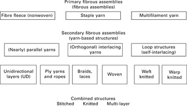
This chapter discusses yarn-based structures, also called secondary fibrous assemblies, which consist of one or more types of primary fibrous assemblies. During the simulation of such structures, the most common and effective approach at present is to regard the yarn as a body with certain material parameters and not as a structure. This simplifies and speeds up simulations significantly. Emphasis is given to geometrical methods for simulation of woven and knitted structures. The simulation of braided structures is presented in two ways. From the structural view, they are similar to woven structures; hence, the same geometric methods can be used for their simulation. For process simulation, separate methods have to be used. Figure 8.1 gives an overview of the classification of the most common textile structures.
The simulation of textile structures aims at the prediction of their properties and behaviour prior to production of the structures themselves. Depending on the application, the important parameters (e.g. geometrical, mechanical, thermal, acoustic etc.) of the structure have to be known and selected so that the customer requirements are met in the best possible way. This is the first objective of the simulation of textile structures − to predict the structure’s properties, giving some approximation for their values, e.g. elasticity modulus, area density, porosity. A typical example is shown in Fig. 8.2: if the calculated water permeability of the convertible roof of the car is lower than the required value, then the roof will most likely be able to shield the passengers in the car from the rain.

8.2 Example of a convertible roof: (a) as a protection against the rain only the water resistance of the structure is required; (b) to be happy with the folding, the complete folding process has to be investigated.
In more complex cases, such as the folding of a cabrio roof, single parameters like water permeability, bending ridigity and thickness alone are not sufficient to make an accurate prediction whether the folding will work properly. In these cases, the complete folding behaviour has to be investigated, for instance using numerical simulation. This explains the second (final) objective of the simulation − to be a tool for the investigation of the complete behaviour of textile structures under certain conditions. The simulation of the complex behaviour of textiles requires information about their structure. In the case of yarn-based structures the most important aspect is yarn geometry. The interlacing between the yarns determines the behaviour, the freedom of the motion and the friction between the yarns.
Feeding the geometry of the yarns into software packages, different simulations are possible:
• with the finite element method (FEM), mechanical, thermal, acoustic and other simulations are possible;
• with computational fluid dynamics (CFD) software, the simulation of the flow of air or moisture through textiles is possible;
• applying dynamics software (mass-spring systems, particle models, etc.), drape and motion behaviour can be simulated.
Because all these simulations cannot be performed without defining the geometry of the relevant structures, the geometry of yarn structures is the main objective of this chapter.
8.2 Principles of geometrical and mechanical modelling
The simulation of textile structures is based on establishing a model to represent the most important behaviour of the structure. In the case of experimental simulations, the working conditions are reproduced using a real model, e.g. of a car, which will be crashed against a wall to simulate impact behaviour. Such simulations are not the objective of this chapter. Here, only computer simulations based on mathematical models are considered. The mathematical models can represent the equations of deterministic physical models (e.g. FEM, mass-point systems, beams), heuristic models, e.g. fuzzy logic, neural nets, genetic algorithms and others, or a combination of these methods.
Heuristic models, based on fuzzy logic and neural nets are described in separate chapters of this book. These can also be applied for the simulation of fabrics. However, their design for different textile structures is in most cases connected with large sets of trials by the researcher, until a suitable neural net architecture or membership functions for a fuzzy logic system are found.
This chapter will therefore concentrate on deterministic models of textile structures (Fig. 8.3). The common way to build simulation models for all yarn-based structures starts with the design of the yarn geometry. There are different ways of constructing this yarn geometry:

• reconstruction from micro-computer tomography images, microtom images, or a series of cross-sections;
• (topological) generation of the geometry, based on the information of the interconnections between the yarns;
• simulation of the production process and calculation of the resulting yarn geometry.
All these approaches are widely used and applied in different cases, depending on the final goal. A brief comparison between these methods is presented in Table 8.1.
Table 8.1
Methods of geometry generation
| Advantages | Disadvantages | |
| Image reconstruction, image analysis | Very exact path reconstruction Suitable for verification of the results from the other models |
Very time and/or cost intensive, Requires special techniques Results are not applicable to other structures Very small pieces of the structure can be analysed |
| Production process simulation | Can produce any kind of patterns with nearly exact path | Computationally intensive Large and complex models – the entire machine and the yarns have to be modeled Requires time, especially for large numbers of repeats In several cases, the resulting accuracy is not needed |
| Topological generation | Suitable for building parametric models for similar structures, fast and inexpensive | Not very exact path reconstruction, requires (mechanical) corrections Limited to the implemented structures |
The use of image recognition is not really connected to any kind of textile structure (Wirjadi, 2009; Wirjadi et al., 2009). Its algorithms work very well for a wide range of structures, if the device that makes the images is able to distinguish the fibres or yarns from the surroundings so that, during the processing of these pictures, these fibres or yarns can be described. One of the difficulties of the use of such models is the detection of the boundaries between the single yarns, especially in those cases where the tows are parallel. The methods used in these cases are extensively discussed in books on image processing and are hence not a topic in this chapter. An example of a MicroCT is of braided structure, used to verify the simulation of the geometry of a rope is shown in Fig. 8.4.

8.4 MicroCT of braided rope. (courtesy of Fraunhofer Institut for Techno- and Wirtschaftsmathematik (ITWM) − Kaiserslautern)
Another method for the creation of the geometry of yarn structures is based on an integrated simulation of the entire production process. This requires understanding the yarns, the motion of the main machine elements and how they interact with the yarns (needles, heald frame drives, beat up, etc.) and an accurate description of the contact pairs (yarn to element, yarn to yarn). In this case, several effects of the production process can be investigated and any structure which can be produced on the modelled machine can be generated with the same model. The disadvantage of this approach is its complexity and the large computing time required.
A third way for the simulation of the geometry of textile structures is based on the existing knowledge about the interlacing between the yarns in the structure. In each of the sub-areas, e.g. weaving, knitting and braiding, systems exist to encode these intersections into a pattern. Using this code representation of the pattern, yarn and machine parameters, the structure can be rebuilt in the computer. This method is relatively simple to implement and applicable to all textile structures. The main disadvantage is that the geometry is idealized and normally requires additional ‘improvement’ so that the yarns are put into a position that corresponds more closely to reality. This third method is discussed in the next section.
Independent of which method is used for geometry generation, the yarns are converted into finite element meshes (see Chapter 6). These can then be used for mechanical simulation using FEM or a simulation of the fluid flow through the structure using CFD (see Chapter 5). In the case of impregnation of the structure inside a resin matrix, the homogenization method can be used as well to predict the equivalent elasticity parameters of the resulting structure.
A completely different approach is normally used for the simulation of a textile structure at the macro-scale. In this case, the generation of the yarn geometry is usually omitted and the surface is considered to be a shell or a plate (see Chapter 6) or a mass-spring system. In these cases, the main question is which kind of material properties have to be used in order for the simulated structure to react in a similar way to the original. Some references discussing such simulations are given in Section 8.7.
8.3 Simulation of wound packages
A well-prepared wound package (e.g. a bobbin) can exist as a body without any core. Wound packages are normally not classified as textile structures because they are used mainly as a ‘preliminary product’ for the production process. There are also several applications where wound packages are the final preform, e.g. in the composites winding of high pressure bottles. Because their properties (e.g. density, density distribution, permeability, stability, stress distribution) are very important for subsequent production processes, their modelling will be considered as well as those of woven, knitted and braided structures. Like other textiles, a bobbin can be simulated in meso- scale (winding level) or in macro-scale (layer by layer).
8.3.1 Simulation of bobbins at the winding level
The relations between the yarn guide motion and the bobbin form have been analysed by, for instance, Efremov and Efremov (1982). Several properties of bobbins in relation to the winding structure are described in detail by Simon and Hubner (1983). A method for calculating the yarn path for the filament winding of composites has been developed (Johansen et al., 1998; Koussios et al., 2004a; Li et al., 2005). Application of this method is reported in Kyosev et al. (2006b).
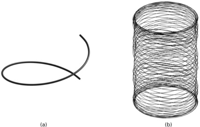
The winding structure (Fig. 8.5b) consists of single windings (Fig. 8.5a), which are stored in the computer as a list of coordinates (ri, φi, zi) of the approximately equally distributed points of the yarns (Fig. 8.6). These coordinates can be obtained by means of experimental measurement or numerical simulation. Within the numerical approach, the coordinates of winding points are calculated from geometrical considerations about the yarn guide motion and the parameters of the winding body.
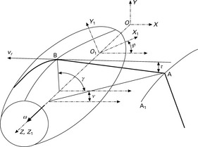
The bobbin is assumed to have a certain geometry, which can be described by the rotation of one or more (piecewise) analytically describable plane lines about the OZ axis. In the industrial case, this is usually a single line, but there also exist winding forms with a more complex geometry not described here. The bobbin body rotates about its OZ axis with an angular velocity w (Fig. 8.6). If the free length AB of the yarn between the yarn guide A and the winding point B is very small, then the winding form is almost completely controlled by the yarn guide, here represented by point A. The influence of this free length can be ignored. It can be assumed that the Z-coordinates of points A and B are the same or the yarn guide moves close to the bobbin surface (AB = 0). In those cases, where the influence of the distance AB needs to be investigated or is more significant, additional geometric relations according to Efremov and Efremov (1982) or Koussios et al. (2004a, 2004b) have to be used for the description of the relation between the yarn guide motion and the winding point.
The simplified case (AB = 0) is often preferred in industrial applications, because of the good control over the bobbin. Then, the following simple algorithm can be used:
a) bobbin surface R(φ, z) as function of the angle and z-coordinate
1. Calculations. For each actual time t t = ti-1 + ![]() t, if ti < tEND calculate:
t, if ti < tEND calculate:
a) the angular position of the current winding point φ = φi—1 + ω. ![]() t, which corresponds to the rotation of the bobbin for the angle
t, which corresponds to the rotation of the bobbin for the angle ![]() φ = w.
φ = w. ![]() t
t
b) the z-position of the yarn guide eye from its motion low zi = Z(ti)
c) calculate the radius at the winding point ri = R(φi, zi) + yarn diameter, as a radius, corresponds to the bobbin surface to the coordinates (φi, zi)
Figure 8.7 shows the results for three simulated bobbins when using this algorithm, with very small differences in the winding ratio nW = nB/nG. According to Simon and Hubner (1983), nW stands for the number of windings per yarn carriage stroke, represents the bobbins revolutions per minute and nG is the number of yarn guide cycles per minute.
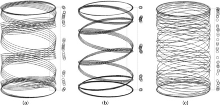
8.7 Examples of simulated winding structures with presentation of the cross-cut section of the layer: (a) precise winding; (b) bad layers − the new windings are positioned directly over the previous ones; and (c) random winding.
The ratio nW = 7.9808 is very close to a whole number and can thus lead to a defective package (Fig. 8.7b). The value nW = 7.9365 can be used for controlled (precise) winding if the distance between the yarns corresponds to the yarn thickness (Fig. 8.7a). The ratio nW = 7.8496 results in a layer with random winding used by drum winding (Fig. 8.7c). On the right side of those figures with windings, their cross-sections through a radial surface are shown, where each circle presents a single yarn cut. These cross-sections show the distribution of the yarns in the layers. Inside the simulated layer (this is not valid for the entire body!), the structure presented in Fig. 8.7c has the most uniform distribution of the winding, at lower density. The windings presented in Fig. 8.7a for a controlled package normally have a higher density compared to the other types. The structure in Fig. 8.7b shows a very high concentration of the windings in very narrow regions, which corresponds to a defect bobbin.
The structures depicted in Fig. 8.7 can be produced by applying very small changes of the winding ratio or the winding angle, but they have completely different densities and mechanical properties. If the simulation is continued for a longer period of time, the surface of the bobbin in Fig. 8.7b will no longer be cylindrical or smooth, but of a more complex form. This surface then has to be stored in the computer so that it can be used for the calculation of the coordinates of the point.
The algorithm shown here does not take into account the influence of the windings on the layer radius. In order to do this, the yarn thickness and the orientation of the yarns have to be considered by determining every single contact point between the windings. such an algorithm is of course possible, but it will work fast and with sufficient accuracy only for windings with a random structure like those depicted in Fig. 8.7c.
When the windings from a half-cycle of the yarn guide intersect the windings from the previous half cycle, the contact geometry is similar to that presented in Fig. 8.8a. In all other cases, where the structure is similar to the one presented in Fig. 8.7a,b, the contact geometry can be defined as a ‘contact line’, not as ‘crossing point’, because a certain length of the yarn segments will touch each other side by side (Fig. 8.8b). This case is not critical, if a segment can be found one level below, which lies across (Fig. 8.8c), as it will determine the radius of the new yarn segment. In many cases, both the yarn segments on the previous layer will have the same orientation as the new one. The calculation of the exact position of the new yarn segment then leads to the contact problem of three-dimensional bodies, which takes more computational resources.

All these relationships can be implemented in a simulation algorithm, which can be used to calculate the yarn shapes with a reasonable degree of geometrical accuracy. However, up until this point, the algorithm does not take into account any mechanical interactions between the yarns. The friction between yarns, the yarn tension during winding and the deformation of the bobbin under the pressure of the windings have to be considered as well if such simulations are to be realistic. For many applications though, a geometry simulation is fully sufficient, e.g. if the yarn guide movement is to be analysed or if the stability conditions of single windings have to be checked.
8.3.2 Stability of the windings
The distribution of the yarns in a thin layer can be simulated using the algorithm described above. Besides using the coordinates of the points, the winding angle α for each yarn segment can be calculated. This angle can be used for checking the stability conditions of the yarn piece (Proshkov, 1986):
where θ is the geodesic angle of the surface and tan εmax = μ is the friction coefficient between yarn and winding surface, T1 and T2 are the yarn tension on the both edges of the winding between the angles 0 and ψ. Here we have to emphasize that, because of the roughness of the surface, the friction coefficient μ is not always equal to the friction coefficient measured for yarn-yarn contact. Equation [8.1] can be used to check whether the windings in the simulated structures are stable or not. In addition, the maximum winding tension T2, ensuring that single yarn segments remain in static equilibrium (stable) over the surface, can be also calculated.
8.3.3 Stress distribution inside wound package
Knowing the stress distribution in the bobbin explains many bobbin properties. Incorrect winding tensions can cause a loss of stability of the package, making it unusable. For synthetic mono- and multi-filament yarns, a higher stress can lead to a deformation of the tube. For certain yarn types, the stress they experience in storage is significant, because different relaxation processes in the layers can cause defects and hence a poor quality of the product at the next processing step. An example of a bobbin where the inner layers are deformed is shown in Fig. 8.9.
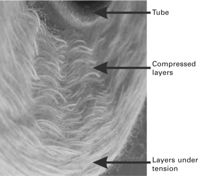
Figure 8.10 shows the three different types of layers used in building the mathematical model of the stress equilibrium of the wound package. The difference between the layers is in their boundary conditions. The innermost layer has a fixed inner radius and the outermost layer has a known outer radius and no pressure from the outside. The mathematical model for the stress distribution is based on the static layer equilibrium. The model is identical to the one presented for the roll making operation by Ghosh et al. (1991b). It is based on the stress equilibrium of single elements in radial direction, with
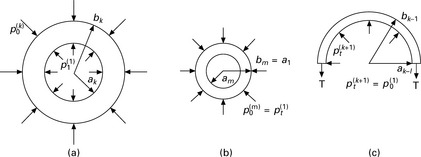
8.10 Layers of a wound package and their boundary conditions: (a) each middle layer is pressed from the inside and the outside; (b) the innermost layer has a definite inner radius and pressure from the outside; (c) the outermost layer has a known outer radius, but is pressure-free from the outside.
where σr and σθ and are the radial and circumferential stresses, respectively. The relations for the strains in terms of radial displacements u can be described
The circumferential elasticity module takes into account the initial yarn elasticity module as well as the winding angle β and the number of yarns in the layer, hence
The pressure–thickness curve of the textile yarns and structures is nonlinear (van Wyck, 1946; Grishanov and Lomov, 1997) (Figure 8.11). As a result, a bi-linear approximation can be used as was shown by Kyosev et al., (2006a, 2006b). Here, a linear stress–strain relation in radial direction
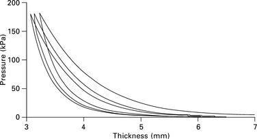
8.11 Example of the experimentally measured values of thickness–pressure curves of layers (three cycles) (Kyosev et al., 2006b).
is used. According to the current deformation εr of each layer, the corresponding elasticity module is then given by
This approach significantly simplifies the equation, but leads to a higher number of iterations if the calculated state is near the deformation limit ![]() .
.
When applying ![]() , we need to solve the following ordinary differential equations for each layer
, we need to solve the following ordinary differential equations for each layer
which has the analytical solution
Here, C1 and C2 are integration constants, which are found for each layer according to the following boundary conditions:
• inside of the first layer (tube deformation is neglected)
• common boundary between layers i and i + 1:
where n is the number of yarns in layer cross-section and F is the winding tension.
Equations [8.12]–[8.15] make up a linear system for the integration constants of each layer, which can be solved in any programming environment by Gaussian elimination. The calculation of the whole body is carried out according to the following algorithm:
0. Initialize the first layer.
1. Build the next layer near the last one and calculate the new equilibrium state for all layers.
2. Calculate stresses, update the geometry of the layers by applying the displacements. Go to step 2 until the complete body is simulated.
Some examples for the calculation of radial and circumferential stresses in a bobbin with radius 0.1 μ are presented in Fig. 8.12. It shows that, after winding of about 10 layers, the yarn inside these layers is no longer under tension (circumferential stress is near zero) and there is a potential risk of loss of stability or producing of a defect body, as shown in Fig. 8.9. It has to be noted that a higher anisotropy rate K can lead to an overflow problem by the calculation of the displacements, for instance for voluminous yarns.

More details about mathematical models for the simulation of the stress–strain distribution inside wound packages of filament winding and for warp beams can be found in Batra et al. (1976), Vicentini (1969), Neal (1967), Beddoe (1967), (Kempner and Hahn (1995), Ursiny et al. (1995), Ursiny (1986) and Koltze (2001). From a mathematical point of view, the stress–strain distribution of the wound package and of fabric rolls presented by Ghosh et al., 1991a,1991b) and, Ghosh and Peng (1995) is identical. The differences are mainly in the mechanical properties of the layers.
8.4 Simulation of woven structures
Woven fabrics are the most thoroughly investigated textile structures. There are over 200 research papers covering different aspects of the geometrical modelling of woven structures. There are several different types of simulations of woven structures, depending on the final goal. The main simulations reported in the literature can be classified into the following groups:
• simulation of the woven fabrics as a structure from an aesthetic or artistic design/colour perspective;
• simulation of the three-dimensional woven structure for further use in mechanical, thermal and other engineering calculations or as well in artistic design;
• simulation of the drape behaviour of the structure, for the purpose of clothing simulation or for the draping of reinforcement textiles for composite parts.
Each of these simulations requires different methods and will be discussed in separate sections. There are also simulations using soft computing techniques which are not discussed here.
8.4.1 Simulation of woven fabrics for artistic design
These simulations are probably the earliest commercially available simulations of woven structures, developed to replace the sophisticated work of designers, preparing punch cards for Jacquard machines. All these simulations start from the weave pattern definition, since it contains the information about the appearance of the yarns from both sides. The usual pattern definition for single layer structures uses the marking black (or 1, if matrix form is used) of these crossing points between the warp and weft yarns, where the warp yarn lays above the weft yarn (Fig. 8.13).
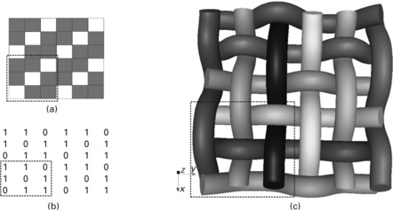
8.13 Coding of woven structures and its simulation: (a) pattern with the marked repeat; (b) the same pattern in matrix form; (c) simulated with the software TexGen (University of Nottingham, 2011) woven structure, corresponding to this pattern.
This coding is used for the control of the heald frames or the Jacquard unit of the weaving machine, as well as for the reconstruction of the geometry of the woven fabric. The places marked with a ‘1’ are those where the warp yarns are visible on the upperside. On the other places, only the weft yarn is visible, whereas the warp yarn is hidden. This principle was and is still used by most computer programs to simulate the appearance of the woven structure, without having to reconstruct the real appearance of the fabric. Using pictures of real or created yarns, appropriately placed and rotated, it is possible to present a realistic view of the structure. Figure 8.14 shows a view of the pattern editor in Arahne© software, whilst Plate XV (see colour section between pages 152 and 153) shows the simulated fabric using the same software. This example is only for demonstration. Nowadays, most programs provide a visual representation of the fabric. A list of currently known programs for weaving simulations is given at the end of this chapter.

8.14 Pattern editor from Arahne (Arahne, 2011).

Plate XV Simulated fabrics by Arahne (Arahne, 2011). Courtesy of Arahne company http://www.arahne.si/.
8.4.2 Simulation of a three-dimensional woven structure
Another, more intuitive way to simulate woven structures is to generate the entire yarn geometry in three-dimensional space and to visualize this, including lightening, shadows, etc. This method is described in this section. There are several research papers which include a mathematical description of the yarn geometry of woven structures in three-dimensional space.
Such mathematical models are based on the description of the yarn path on its plane. In the plane of a warp yarn path, the weft yarns are shown with their cross-section form and this allows the definition of the contact points and the types of the lines between them. Figure 8.15 demonstrates one of the simplest and earliest models (Peirce, 1937) of a woven structure based on a circular cross-section of the yarns and modelling of the yarn path using circular arcs and lines. This model has been extended in several papers for different shapes of the yarn cross-section (lenticular, eliptic) and for different kinds of approximations of the yarn paths (eliptic, parabolic, cubic, natural splines, etc.). Experience shows that each of these models can be valid for certain cases but are not applicable to other cases. For plain fabrics, a typical model can be found in Behera and Hari (2010) and Postle et al. (1988). A very precise implementation of the different models in a software program which chooses the suitable yarn path approximation function depending on the yarn cross-section form is the program WiseTex© (Lomov et al., 2011).

8.15 Principle of the calculation of the yarn axis coordinates in the case of yarns with circular cross-section and approximation of the yarn paths using circular arcs and lines.
In this section, only the basic steps for modelling are described, based on the definition of the key points and connections. It is possible that, in some regions, the yarns are interpenetrating, whilst in other regions, they are more widely spaced. However, a refinement of the yarn path segments at some later stage is always possible. Starting from the pattern coding, and using the yarn cross-section dimensions, the axes of the yarns can be calculated. The first warp yarn on Fig. 8.16 starts with a position underneath the weft yarn. After that it lays twice above the weft yarns. For simplicity, it can be assumed that the undulation of the yarn axis is equal to the yarn diameter, so that h is equal to the yarn radius on Fig. 8.16. This leads to


with Matr representing the coding matrices with the pattern and i and j standing for the indices of its rows and colomns, respectively.
The x-coordinates of the warp yarns depend on their position and the space between the yarns. For the case of equally distributed warp yarns with the distance twrap between them, the ith warp yarn has the x-coordinate:
The key-point, where this warp yarn is above or underneath the weft yarn number j, has the y-coordinate:
where the distance between the weft yarns is tweft.
Similarly, the coordinates of the weft yarns can be calculated and so a list of coordinates for each yarn path can be calculated in the form
Using this set of coordinates, the yarn axis can be created using a suitable kind of connecting functions between the points, as presented in Fig. 8.17a. Around this yarn axis, a yarn volume is built, and the yarn cross-section around a set of points of the yarn axis is calculated (Fig. 8.17b). Each crosssection has to lie on a plane, spanned by the normal and the binormal vector to the yarn path at that point. For a FEM calculation with volume elements, the entire yarn volume has to be meshed using small elements, as in Fig. 8.17c. More details about the algorithms for interpolation of the yarn axis, building the yarn volume and meshing can be found in Sherburn (2007) and the software package TexGen (University of Nottingham, 2011). After the geometry is created in this way and uploaded into FEM or CFD software, different behaviours like mechanical, thermal, fluid dynamics, etc. can be simulated. Another use of this geometry is mapping of images from real yarns to the surface of the yarn in order to achieve a photorealistic appearance for the artistic design of the fabrics. In this way it is as possible to create realistic pictures of plush structures, as for instance by EAT GmbH ‘The DesignScope Company’ (EAT, 2011).
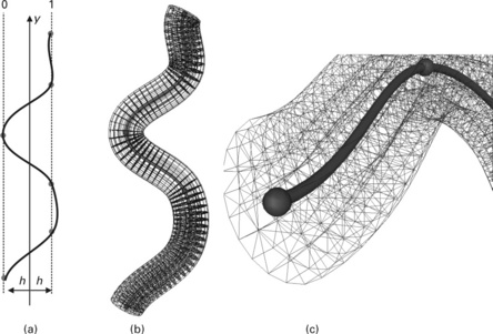
8.17 a)–(c) Extrusion of the yarn cross-section around the axis and meshing its volume, here using TexGen (University of Nottingham, 2011).
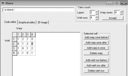
The preparation of the geometry of multilayer woven structures works in a similar way. The pattern coding for multilevel structures in this case is based on a matrix with numbers, each marking the level on which one warp yarn crosses the weft yarns (Plate XVI and Fig. 8.18). Figure 8.19 shows the topological representation of the woven structure based on the assumption that the weft yarns are straight (Fig. 8.19a) or bent at the crossing places with the warps (Fig. 8.19b). The crimp calculations need to be undertaken after the mechanical data of the yarns has been provided.

The method described here is suitable for the simulation of an approximate geometry of the yarn structure. The simulation of the exact geometry of the woven structure is not possible using only pure geometrical data of the pattern and the yarns. The geometry of the yarns depends significantly on their bending rigidity, the twist as well as the conditions during weaving. Because of this, only simulations which take into account all this information are able to reproduce the geometry of the woven structure correctly. Currently the only program which takes into account the mechanical parameters of the yarns is WiseTex (Lomov et al., 2011). Other programs only cover geometric data.
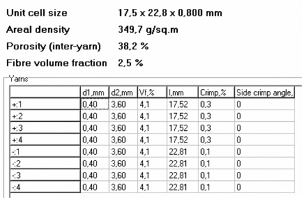
Usually the calculations for static cases are based on the principle of the minimum of the potential energy of the structure, in this case of all yarns (Verpoest and Lomov, 2005; Lomov et al., 2006). The following example demonstrates some results of the simulation of the tensile and lateral compression behaviour of a woven structure using WiseTex. A woven structure (Heuwinkel, 2011) with the following parameters is simulated:
• warp yarn fibres: polyester (PES) filaments; fineness 0.13 tex, diameter 0.022 mm;
• weft yarn fibres: PES filaments, fineness 0.39 tex, diameter 0.021 mm;
• warp yarn parameters: fineness 21 tex, modelling diameter 0.3 mm, 153 filaments in cross-section, without twist, bending stiffness 0.068 N/ mm2; strength 6 N, maximal elongation 25%, cross-section compression parameters η1 = 0.812, η2 = 1198,
• weft yarn parameters: fineness 71 tex, modelling diameter 0.54 mm, 182 filaments in cross-section, without twist, bending stiffness 0.17 N/ mm2; strength 6 N, maximal elongation 26%, cross-section compression parameters η1 = 0.812, η2 = 1.188;
• fabric parameters: 60 warp yarns per cm; 9 weft yarns per cm; thickness 0.5 mm; width 10 mm; plain woven pattern.
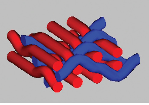
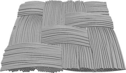
The force–elongation curve from an experimental test and from the simulation of the tension behaviour with WiseTex is presented in Fig. 8.20, where it can be seen that the trend of the curves is the same with a small underestimation of the tension by WiseTex. The simulated compression curve has a similar trend as the measured one, but its values are several percent smaller (see also Fig. 8.21). These differences are a result of the differences of the behaviour of a multifilament yarn compared to a monofilament yarn. For the geometrical modelling, the yarns are presented with a constant cross-section which in reality is not constant. Figure 8.22 presents a view of a similar structure and the modelled unit cell is presented in Fig. 8.23.
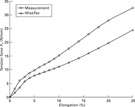
8.20 Simulated and measured load elongation curves of a woven tape (Heuwinkel, 2011).
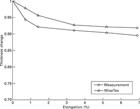
8.21 Simulated and measured compression curves of a woven tape (Heuwinkel, 2011).

8.22 Photograph of a similar structure as the one modelled. The multifilament yarns without twist change their cross section on the places where there is no contact with the neighbouring yarns.

If the yarn geometry has to be presented properly, the yarn cross-section has to be variable. In the case of staple yarns, the yarn volume density has to be variable. Such options are currently not implemented in the available software. One solution is to model the yarns with a constant cross-section, allowing penetration between these, but keeping the proper number of single filaments and the mechanical data (Fig. 8.23) constant. For mechanical calculations based on yarn path geometry, this approach leads to a good approximation of the experimental data as in the example shown. If fluid transfer between the yarns has to be simulated, such interpenetrations between the yarns can lead to more significant differences between the simulation and experimental results.
If the yarn level modelling of the woven structures is not sufficiently precise for an application, then the yarns have to be modelled on the filament level. This approach solves the problem of the differences in the cross-section and avoids the need to investigate the in-plane behaviour of the yarn crosssection. However, this requires significantly higher computational resources and a larger preparation time for the samples (Durville, 2010) (Fig. 8.24). A key disadvantage to all the current programs for the simulation of the woven structure is that they require some kind of topological representation of the structure. This is generally not the same as the pattern for the weaving machine, especially for multilayer structures. Some special algorithms for hollow or angle interlock structures, where the simulation of the structure is based on the coding for the machine, are implemented by TexEng LTD (TexEng Software Ltd, 2011b) and Plate XVII presents an example graphical interface for a hollow structure.
8.24 Modelled woven structure with twill pattern, where the single yarns are presented as a set of filaments, modelled completely (Durville, 2010).

8.5 Simulation of braided structures
The unit cell (smallest repeat) of braided structures is identical to those of woven structures. Because of this, the methods for the simulation of the braided structures are very similar to those used for woven structures. Due to several significant differences during the production process (e.g. beat up force during weaving which does not exist in braiding), braided structures are not as dense as woven structures and have different mechanical behaviour.
8.5.1 2D colour pattern design of braided structures
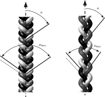
Only the areas where one yarn is visible from the upper side show the colour of the yarn. As a result, only the colours of the yarns on the top side of the interlacing are important for the colour pattern design of braided structures. The principle of pattern calculation is identical to that of woven structures, described in Section 8.4 (Fig. 8.25). Braided structures are built by one, two or more systems of yarns which interlace with each other or with other systems at a certain angle. Half of this angle is usually equal to the angle between the yarns and the product axis and is called the braiding angle (Fig. 8.26). The braiding angle is important for the realistic simulation of the fabric’s appearance.

Owing to the lower number of products and customers, the use of CAD for braided products in the fashion area is uncommon. There is no software which simulates braided structures photorealistically, unlike woven and the weft knitted structures. For most customers, the distribution of the colours is sufficient in order to check from the simulation if the product meets their requirements. Figure 8.27 shows a simulation of one sample with a diagonal colour effect with three different braiding angles, using CAB software from Herzog (Herzog Maschinenfabrik, 2011).

8.27 Tubular sample with diagonal colour effects, yarns in 'two over two' (diamond) arangement, simulated with different braiding angle using CAB Design from August Herzog GmbH and Co. KG (Herzog Maschinenfabrik, 2011).
Since the patterns used in the braided samples are very limited, with fewer than five commonly used patterns, it is not necessary to calculate the pattern matrix for tubular and flat structures as for woven structures. After determining whether the structure is flat or tubular, and selecting the type of yarn interlacing (one over one, two over two, diamond = two over two but with two ply yarn), the algorithms for the simulation of the structure are identical. Figures 8.28 and 8.29 show the graphical user interface for patterning of tubular and flat braided fabrics respectively using CAB Design software, where the user can choose the colour for one yarn (= carrier). After picking the number of carriers, the places where this yarn will be visible are automatically coloured in the chosen colour.

8.28 Graphical user interface for simulation of tubular braided fabrics, using the CAB Design software by August Herzog GmbH & Co. KG. (Herzog Maschinenfabrik, 2011).

8.29 Graphical user interface for the simulation of flat braided fabrics, using the CAB Design software by August Herzog GmbH & Co. KG (Herzog Maschinenfabrik, 2011).
It is apparent that the simulated view of the structure is not significantly different from the pattern view in Fig. 8.25c, where the yarn colours, braiding angle and positions of the yarns in the product are shown. If one yarn floats first above two other yarns and then underneath two yarns, this floating is presented as a rectangular area equal to the two squares without showing the square borders.
8.5.2 3D design of braided structures
Reports of algorithms and software for the creation of 3D yarn geometry of braided structures can be found in several papers. These works can be divided into three groups:
• simulation of the yarn geometry for flat and tubular structures;
• simulation of the geometry and the shape of the braid during overbraiding of certain profiles;
The geometry of flat and tubular structures can be simulated using the same principle applied to woven structures using geometric methods (Liao and Adanur, 2000; Kyosev, 2007). This is a sufficiently accurate representation for several applications and in establishing the initial geometry for FEM computation. Figure 8.30 shows simulated flat braided structures with different numbers of carriers whilst Fig. 8.31 shows simulated tubular braided structures using TexMind software (TexMind UG, 2011).

8.30 Simulated 3D geometry of flat braided structures from machines with (a) 3, (b) 5 and (c) 17 carriers (Kyosev, 2011).

8.31 Simulated 3D geometry of tubular braided structures from machines with (a) 8, (b) 16 and (c) 32 carriers (Kyosev, 2011).
The simulation of overbraided products is more complex then tubular and flat braids. This is due to the yarn path depending on the mandrel shape and in several cases on the dynamics of the braiding process. In these cases, purely geometric methods can be used, if the braided structure is ‘open’, i.e. if the neighbouring yarns work in the same direction and do not come into contact with each other. studies by Rawal et al. provide a good description of the yarn paths which can be used for simulation during the overbraiding of different regular bodies, either as a pyramid (Rawal et al., 2007), cone or cylinder (Rawal et al., 2005) or in the case of triaxial structure (Potluri et al., 2003). If the braid has a higher density and the yarns are near to each other, then the geometric methods lead to larger differences in the path positions of the yarns and can be used only as a visualization method.
8.5.3 Simulation of braided structures using process simulation
The simulation of the braiding process and the braids themselves is based on the analytical description of the yarn paths during the braiding process. The contact between two yarns has to be detected to allow calculation of the contact points between the yarns. The differences in the approaches of different researchers are in the treatment of the crossing points between the yarns. Different models exist for cases where the yarn remains on its initial place or moves, for friction between the yarns, friction between yarn and mandrel and how the yarn cross-section is modelled.
In the most common examples, the yarn axes are used for the calculations and friction is ignored. Examples of the use of this method in the case of triaxial braided structures can be found, for example, in Zhang et al. (2007). The analysis of local changes of the braiding angle in the structure, depending on the mandrel profile during the overbraiding process, can be found in Nishimoto et al. (2010). In this paper, the yarn path between the last braiding point, the current contact points over the mandrel and the carrier are described. The same principles, built into a more general algorithm and software for overbraiding simulation, are presented in Akkerman and Rodriguez (2006) and Kessels and Akkerman (2002). In these studies, the mandrel geometry is presented as a discrete (meshed) surface and the contact between the yarns and the elements of this surface is calculated in order to establish the final position of the yarn pieces. Current FEM software can also be used. As an example, the carrier arrangement and motion for a 3D braiding machine from August Herzog Maschinenfabrik GmbH is simulated prior to actual operation using special simulation software, which tests the collision control and path of the carriers (Plate XVIII). The resulting geometry from such a simulation is presented in Plate XIX (Stueve and Gries, 2009). The simulated geometry can also be used for predicting the properties of the braids using FEM or other methods with suitable boundary conditions and loads (Pickett et al., 2009). In order to speed up the simulation process, the yarns are modelled with a constant cross-section. Once proper properties of the yarns in the lateral direction have been determined and defined prior to the simulation, this method can produce simulated structures which are very close to reality.
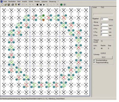
Plate XIII Software for simulation and control of the braiding process on a 3D braiding machine of August Herzog Maschinenfabrik, used by ITA of RWTH Aachen University (Stueve and Gries, 2009).

Plate XIX Simulation of the overbraiding of a body using explicit FEM Software PAM-CRASH (Stueve and Gries, 2009).
8.5.4 Simulation of the properties of braided fabrics
The geometry of the braids is not only used to visualize the braided structure, but is also a necessary step for the prediction of the mechanical and other properties of the braids. Some basic geometric calculations for tubular and flat tubular braids (expected diameter, braiding angle, etc.) can be performed by the CAB Design software mentioned above (Herzog Maschinenfabrik, 2011). Some of the calculations are also shown on the web page of the company A & P Technology (A&P Technology, 2011). The calculation of unit cell properties such as the size of the unit cell, pore size, as well as application of the homogenization method, is also possible using the WiseTex package (Lomov et al., 2006). Figure 8.32 presents the graphical user interface for the preparation of the geometry and material properties of the braided structure. The results for the geometrical properties of the unit cell are presented in Fig. 8.33 and the 3D model of the fabrics in Fig. 8.34.


8.6 Simulation of knitted structures
Knitted structures are built by interlooping of yarns. Depending on the type of the interloping, they can be classified as weft knitted structures (Fig. 8.35c), where one yarn builds loops in the horizontal (weft) direction whilst, in the next row, the same (or a different) yarn closes the loops of the previous row, building new loops. In contrast, warp knitted structures are built from several (warp) yarns, where one yarn builds only one (or two in some structures) loops per row (Fig. 8.35b). In both cases, the loops consist of the same elements − head (H), legs (L) and feet (F) (Fig. 8.35a). The feet connect neighbouring loops in weft knitted structures and loops from different rows in the case of warp knitted structures.
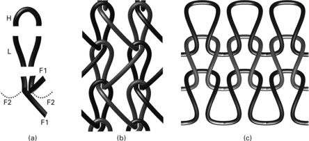
8.35 Knitted structures: (a) elements of one loop; (b) warp knitted structure; and (c) weft knitted structure (Kyosev and Renkens, 2010).
Different mathematical descriptions of knitted loop geometries have existed for more than 50 years (Leaf, 1955), but a detailed description of the loop in the different states of the fabrics still remains an ongoing research problem. The common techniques are:
• to model an idealized geometry and refine it so that some kind of relaxed structure is built;
• to simulate the whole knitting process and create the knitted structure as result of the simulation.
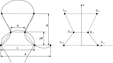
The first method leads to useful results within a very short time and thus is preferred, provided the exact yarn paths are not really necessary. All geometric models for both warp and weft knitted structures in this case are based on the presentation of the loop form (Fig. 8.36) using some key points, usually the projections of the contact points above the plane surface. The exact x and y-coordinates of every key point can be derived using the loop sizes in both directions. Assuming that the yarn cross-section is circular, the z-coordinates of the key-points can also be calculated (Fig. 8.37). More details about the equations for the calculations can be found for instance in Kyosev and Renkens (2010). After calculating the coordinates of the key points, different curve types can be used for their connections. Kurbak and Ekmen (2008) and Kurbak and Soydan (2008) establish very detailed geometrical relationships, though alternative methods using cubic splinces or other approximation functions also work well.
8.36 Knitted structures: (a) elements of one loop; (b) warp knitted structure; and (c) weft knitted structure (Moesen et al., 2003; Kyosev and Renkens, 2010).

8.37 Knitted structures: (a) elements of one loop; (b) warp knitted structure; and (c) weft knitted structure (Kyosev and Renkens, 2010).
8.6.1 Weft knitting examples
Figures 8.38 and 8.39 show 3D simulations of weft knitted structures with WeftKnit and KnitGeo Modeller software. Both programs have been developed in order to generate 3D yarn geometry to allow further calculation. Another kind of simulation of weft knitted structures uses photorealistic techniques. Such modules are based on the visibility of the yarns on the front side and include the structure of the yarns. Figures 8.40 and 8.41 show photorealistic simulations of weft knitted structures using software developed by Shima Seiki (2011). This can show the characteristic hairiness of fancy yarns. There are two ways to produce this simulation:

8.38 3D Geometry of weft knitted structure using WeftKnit (Moesen and Lomov, 2011).

8.39 Geometry of weft knitted structure using KnitGeo Modeller of TexEng Software LTD (TexEng Software Ltd, 2011a).

8.40 Photo realistic simulations of weft knitted fabrics with the software of Shima Seiki. Courtesy of Shima Seiki http://www.shimaseiki.com/.
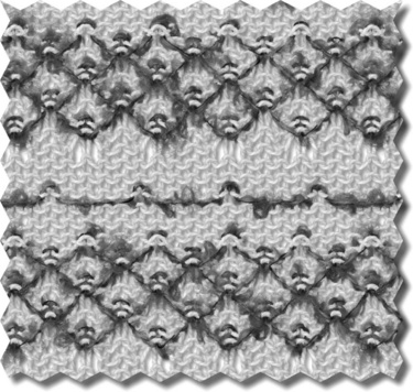
8.41 Photo realistic simulations of weft knitted fabrics with tuck stitches. Courtesy of Shima Seiki http://www.shimaseiki.com/.
8.6.1 Warp knitting examples
Gӧktepe and Harlock (2002) demonstrated a model of a simple warp knitted structures in 3D form, but this was insufficient for industrial use. Robatille et al. (2000) have described a method of modelling reinforced knitted fabrics with significantly thinner and more flexible looping threads than the warp, weft or diagonal yarns (rovings). Both models, however, were developed for a small group of structures only and are thus not suited for more general applications. Current studies of the mechanical properties of warp knitted structures, for instance bending properties by Jiang et al. (1999), are valid only for a certain group of fabrics, and are not generally applicable. Based on the basic method presented at the beginning of Section 8.6, warp knitting simulation tools were developed and reported in Renkens and Kyosev (2007) for single needle bed machines, and Renkens and Kyosev (2011) for double needle bed machines, including spacer and tubular fabrics. Such models are implemented in industrial CAD software packages developed by ALC Computertechnik, Renkens Consulting and TexMind UG (TexMind UG, 2011).
Figure 8.42 shows the difference between the geometrical model (a) and the model after performing a mechanical computation with it (b). The mechanical models in this case can be based on different assumptions, e.g. using trusses and joints or mass-spring systems with contact detection. The basic principles of these models are described in Chapter 6 and can also be found in Kyosev et al. (2005), Kyosev and Renkens (2010) and (de Araujo et al. (2004).

8.7 Future trends
The simulation of the dynamic behaviour of textile fabrics is required for composites forming operations, for clothing simulation and other applications. The drape behaviour of fabrics can be simulated efficiently using mass-spring systems as shown in Han and Stylos (2010), Volino and Magnet-Thalmann (2000) and several other papers. This behaviour requires the material constants of the fabrics such as elastic, shear and bending modulus and area density, which depend on the material used and the woven structure.
Multi-scale approaches integrate the simulation on at least two levels − mezo-level − with the yarn geometry and pattern configuration and macro-level − with the effective fabric data, so that the complete fabric behaviour can be simulated. Such multiscale approaches require more complex computational models and special strategies which allow the material data at the macro level to be updated with the results from simulation at the meso-scale level. Interesting results are presented for instance in Vidal-Salle and Boisse (2010) for woven structures.
Another approach is to represent the single fibre or filaments in the yarns and model their complete behaviour. These models are extremely computational intensive, because several contact detections and calculations have to be performed at every time step; it is well known that contact calculations are time-consuming operations. With increasing computer power, such models are already proving useful, as reported for instance in Durville (2010). Another trend is the integrated simulation of the entire production process, including yarn and fabric deformation and the movement of machine parts which can lead to a simulation of the fabric structure (for instance using FEM; see Chapter 6).
8.8 Sources of further information
Books
The basics of the fabric mechanics can be found in several journal articles. A good overview of the classical methods is given in Postle et al. (1988). A more modern, computational oriented presentation of the theory is given in the Theory Manual of WiseTex (Lomov et al., 2011). A new book, which summarizes the most known methods for the calculations of single layer woven structures is Behera and Hari (2010). The modelling of knitted structures is discussed in a separate chapter in Kyosev and Renkens (2010) and several other modelling aspects for the prediction of the textile behaviour can be found in Chen (2010).
Software for fabrics design and simulation
This is a slightly modified list of the software for weaving, taken from Apparel Research (2011), which gives only an overview about the most programs, and is not exhaustive. It must be noted that some companies have merged in recent years and their products hence appear under new names, while other companies have good products but their web pages are not listed on the top results when searching the WWW in some countries. There are as well several good simulation tools, developed for certain companies, which are reported in some papers, but are not available for a non-licensed user.
| Arahne | http://www.arahne.si/ |
| AVL Looms, inc | http://www.avlusa.com/ |
| Canyon Art | http://www.weaveit.com/ |
| The Design Scope Company (EAT) | http://www.designscopecompany.com/ |
| Information Systems Consultants | http://www.isconindia.com/ |
| JacqCAD International | http://www.jacqcad.com/ |
| Mapple Hill Software | http://www.mhsoft.com/ |
| MüCAD | http://www.mueller-frick.com |
| Point Carre USA | http://www.pointcarre.com/ |
| Porini USA | http://www.porini.us/ |
| Penelope® | www.infotex.es |
| Scot Weave | http://www.scotweave.com/ |
| Startes Jaquard | http://www.startes.it/ |
| TeckMen Systems LTD | http://www.teckmen.com/ |
| Viable Systems Inc. | http://www.viacad.com/ |
| Weave Point | http://www.weavepoint.com/ |
| WiseTex | http://www.mtm.kuleuven.be/Onderzoek/Composites/software/wisetex |
| Y xendis | http://www.yxendis.com/ |
Weft knitting
| FigPaint | http://www.fib.fr/gbsite/ |
| Stoll | www.stoll.com |
| Shima Seiki | http://www.shimaseiki.com/ |
| Steiger Textil | http://www.steiger-textil.ch/eng/profilo.htm |
| WeftKnit | http://liegebeest.studentenweb.org/ |
Warp knitting
| MüCard | http://www.mueller-frick.com |
| TexMind | http://www.texmind.com |
| CADT | http://www.cadt.com/ |
| ALC Computertechnik (now Texion) | http://www.texion.eu |
| EAT | http://www.designscopecompany.com |
Braided fabrics
| CAB Design | http://www.herzog-online.com/ |
| TexMind | hww.texmind.com |
| WiseTex | http://www.mtm.kuleuven.be/Onderzoek/Composites/software/wisetex |
8.9 References
A&P Technology. Braiding calculator, 2011. http://www.braider.com/Resources/Braid-Calculator.aspx [[online]. Available from:].
Akkerman, R., Rodriguez, B.H.V. Braiding simulation for rtm preforms. In: TexComp. 8, 2006.
Apparel Research. Apparel Research, 2011. http://www.apparelsearch.com/software_knitting_and_weaving.htmte [[online]. Available from:].
Arahne. Arahne [online]. Available from: http://www.arahne.si/, 2011.
Araújo, M. de, Fangueiro, R., Hong, H., Modelling and simulation of the mechanical behaviour of weft-knitted fabrics for technical applications: Part III: 2D hexagonal FEA model with non-linear truss elements. Autex Research Journal [online], 2004;4(1):24–32 http://www.autexrj.com/cms/zalaczone_pliki/5-04-1.pdf [Available from: [Accessed July 2011].].
Batra, S., Lee, D., Backer, S. On the stress analysis of cylindrically wound packages: the case of a warp beam. Textile Research Journal; 1976. [June, 453].
Beddoe, B. Anisotropy of yarn on a flanged tube. The Journal of Strain Analysis. 1967; 2:207.
Behera, B., Hari, B.K. Woven Textile Structure: Theory and application. Cambridge: Woodhead Publishing Ltd; 2010.
Chen X., ed. Modelling and Predicting Textile Behaviour. Cambridge: Woodhead Publishing, 2010.
Durville, D. Simulation of the mechanical behaviour of woven fabrics at the scale of fibers. International Journal of Material Forming. 2010; 3(S2):1241–1251.
EAT. Designscope [online]. Available from: http://www.designscopecompany.com, 2011.
Efremov, E., Efremov, B., Basics of the theory of yarn windingRussian. Original title: EɸpeMOB, E.Д, EɸpeMOB, Б.Д. OCHOBLI TEOии HaMaTъIBaHии ииTи Ha ЛaκOBκy. Moskau: Legkaia i pistevaia promislenost, 1982.
Ghosh, T.K., Peng, H. Analysis of fabric deformation in a roll-making operation. Textile Research Journal. 1995; 65(12):739–747.
Ghosh, T.K., et al. Analysis of fabric deformation in a roll-making operation. Textile Research Journal. 1991; 61(4):185–192.
Ghosh, T., et al. Analysis of fabric deformation in a roll-making operation: Part I: A static Case. Textile Research Journal. 1991; 61(3):153–161.
Goktepe, O., Harlock, S. Three-dimensional computer modeling of warp knitted structures. Textile Research Journal. 2002; 72:266–272.
Grishanov, S., Lomov, S.E.A. The simulation of the geometry of two-component yarns. Part I: The mechanics of strange compression: Simulating yarn cross-section shape. Journal of Textile Institute. 88, 1997. [Part 1 (2)].
Han, F., Stylos, G.K. 3D modelling, simulation and visualisation techniques for drape textiles and garments. In: Chen X., ed. Modelling and predicting textile behaviour. Cambridge: Woodhead Publishing; 2010:388–421.
Herzog Maschinenfabrik, A. CAB Design: Computer Aided braid design [online]. Oldenburg, 2011 http://www.herzog-online.com/conpresso4/_data/CAB-Design_en.pdf [Available from:].
Heuwinkel, F. Analyse mechanischer Eigenschaften von Bandgeweben. Hochschule Niederrhein; 2011.
Jiang, J., Hu, J., Ko, F. Characterizing and modeling bending properties of multiaxial warp knitted fabrics. Textile Research Journal. 1999; 69(9):691–697.
Johansen, B., Lystrup, A., Jensen, M. CADPATH a complete program for the CAD- CAE-and CAM-winding of advanced fibre composites. Journal of Materials Processing Technology. 1998; 77(1–3):194–200.
Kempner, E., Hahn, H. Effects of radial stress relaxation on fiber stress filament winding of thick composites. Composites Manufacturing. 1995; 6(2):67–77.
Kessels, J., Akkerman, R. Prediction of the yarn trajectories on complex braided preforms. Composites Part A: Applied Science and Manufacturing. 2002; 33(8):1073–1081.
Koltze, K. Zur Optimierung des Zentrifugenspinnverfahrens durch robustes Prozefi-design. PhD. Technische Universitat Chemnitz; 2001.
Koussios, S., Bergsma, O., Beukers, A. Filament winding. Part 2: Generic kinematic model and its solutions. Composites Part A: Applied Science and Manufacturing. 2004; 35(2):197–212.
Koussios, S., Bergsma, O., Beukers, A. Filament winding. Part 1: Determination of the wound body related parameters’. Composites Part A: Applied Science and Manufacturing. 2004; 35(2):181–195.
Kurbak, A., Ekmen, O. Basic studies for modeling complex weft knitted fabric structures Part I: A geometrical model for widthwise curlings of plain knitted fabrics. Textile Research Journal. 2008; 78(3):198–208.
Kurbak, A., Soydan, A.S. Basic studies for modeling complex weft knitted fabric structures Part III: A geometrical model for 1 × 1 purl fabrics. Textile Research Journal. 2008; 78(5):377–381.
Kyosev, Y., Model generator for tubular braided fabricsIn: Finite Element Modeling of Textiles and Textile Composites. St Petersburg, Russia: Katholieke Universiteit Leuven & St Petersburg State University of Technology and Design, 2007.
Kyosev, Y. TexMind Braid Modeller [online], 2011. www.texmind.com [Available from:].
Kyosev, Y., Renkens, W. Modelling and visualization of knitted fabrics. In: Chen X., ed. Modelling and Predicting Textile Behaviour. Cambridge: Woodhead Publishing; 2010:225–262.
Kyosev, Y., Angelova, Y., Kovar, R. 3D modelling of plain weft knitted structures from compressible yarn. Research Journal of Textile and Apparel, Hong Kong. 2005; 9:88–97.
Kyosev, Y., Reinbach, I., Gries, T. Stability problems of textile wound structures. PAMM. 2006; 6(1):235–236.
Kyosev, Y., Reinbach, R., Gries, G. Virtual bobbin: building; potential and problems. Proceedings in Applied Mathematics and Mechanics. 2006; 6:235–236.
Leaf, G.G.A. The geometry of a plain knitted loop. Journal of the Textile Institute. 1955; 45:T587–605.
Li, H., Liang, Y., Bao, H. CAM system for filament winding on elbows. Journal of Materials Processing Technology. 2005; 161(3):491–496.
Liao, T., Adanur, S. 3D-structural simulation of tubular braided fabrics for net-shape composites. Textile Research Journal. 2000; 70(4):297–303.
Lomov, S., et alIntegrated textile preprocessor WiseTex, Version 2.5: Computational models, methods and algorithms. Leuven, KU Leuven: Department MTM, 2006.
Lomov, S., et al. WiseTex [online]. Available from: http://www.mtm.kuleuven.be/Onderzoek/Composites/Research/meso-macro/textile_composites_map/textile_modelling/textile_modelling_fe, 2011.
Moesen, M., Lomov, S.V. WeftKnit [online]. Available from: http://liegebeest.studentenweb.org/weftknitEN.html, 2011.
Moesen, M., Lomov, S., Verpoest, I., Modelling of the geometry of weft-knit fabrics. Techtextil (Hg.) 2003 − TechTextil Symposium 7–10 April 2003, 2003.
Neal, B. Behaviour of filament yarn wound on a flanged cylinder. Journal of Strain Analysis. 1967; 2:213–219.
Nishimoto, H., et al. Prediction method for temporal change in fiber orientation on cylindrical braided preforms. Textile Research Journal. 2010; 80(9):814–821.
Peirce, F.T. 5 − The geometry of cloth structure. Journal of the Textile Institute Transactions. 1937; 28(3):T45.
Pickett, A.K., Sirtautas, J., Erber, A. Braiding simulation and prediction of mechanical properties. Applied Composite Materials. 2009; 16(6):345–364.
Postle, R., Carnaby, G., Jong, S. de. The Mechanics of Wool Structures Ellis. Horwood Limited, 1988.
Potluri, P., et al. Geometrical modelling and control of a triaxial braiding machine for producing 3D preforms. Composites Part A: Applied Science and Manufacturing. 2003; 34(6):481–492.
Proshkov, A. Mechanisms for yarn winding (topics of design). In Russian. Original title: ЛpoIIIκOB, A.Φ. MexaHиɜMъI pacκЛaДκи ииTи (BoЛpocъI ЛpoeκTиpoBaиия), MocκBa, Лe![]() ЛpoMбъITи3ДaT. Moscow: Legpromizdad; 1986.
ЛpoMбъITи3ДaT. Moscow: Legpromizdad; 1986.
Rawal, A., Potluri, P., Steeleand, C. Geometrical modeling of the yarn paths in three-dimensional braided structures. Journal of Industrial Textiles. 2005; 35(2):115–135.
Rawal, A., Potluri, P., Steele, C. Prediction of yarn paths in braided structures formed on a square pyramid. Journal of Industrial Textiles. 2007; 36(3):221–226.
Renkens, W., Kyosev, Y. Geometrical modelling of warp knitted fabrics. Finite Element Modelling of Textiles and Textile Composites', St Petersburg. 2007; 26–28. [Sept. 2007].
Renkens, W., Kyosev, Y. Geometry modelling of warp knitted fabrics with 3D form. Textile Research Journal. 2011; 81(4):437–443.
Robitaille, F., et al. Geometric modelling of industrial preforms: warp-knitted and multiple layer textiles. Journal of Materials: Design and Applications, Proc. Institution of Mechanical Engineers (Part L). 2000; 214:71–90.
Sherburn, M. Geometric and mechanical modelling of textiles. PhD. University of Nottingham; 2007.
Seiki, Shima. SDS-ONE APEX [online], 2011. http://www.shimaseiki.com/product/design/sdsone_apex/ [Available from:].
Simon, L., Hubner, M. Vorbereitungsmaschinen fur Weberei, Strickerei und Wirkerei. Berlin, Heidelberg, New York, Tokyo: Springer Verlag; 1983.
Stueve, J., Gries, T., Advances in the simulation of the overbraiding process using FEM. SAMPE. SEICO 09: Sampe Europe 30th International Jubilee Conference and Forum, 2009:618–625.
TexEng Software Ltd. KnitGeoModeller [online], 2011. http://www.texeng.co.uk/knitgeomodeller.html [Available from:].
TexEng Software Ltd. Weave Engineer [online], 2011. http://www.texeng.co.uk/2dfabricsl.html [Manchester, Available from:].
TexMind, U.G., Modelling of Textiles with TexMind Software Products − an overview [online]. Monchengladbach. 2011 www.texmind.com [Available from:].
University of Nottingham. TexGen [online], 2011. http://texgen.sourceforge.net/index.php/Main_Page [Available from:].
Ursiny, P. Neue Erkenntnisse uber den Spannungsaufbau in Spulen. Textiltechnik. 1986; 36(10):535.
Ursiny, P., Hes, L., Magel, M. Vergleichmafiigung des Spannungsaufbaues in Spulen. Meliand Textilberichte. 1995; 76(5):314–315.
van Wyck, C. A study of the compressibility of wool, with special reference to South African merino wool. Oderstepoort Journal of Veterinary Science and Animal Industry. 21(99), 1946.
Verpoest, I., Lomov, S.V. Virtual textile composites software WiseTex: integration with micro-mechanical, permeability and structural analysis. Composites Science and Technology. 2005; 65(15–16):2563–2574.
Vicentini, V. Calculation of the elastic deformation of textile beams during winding. Journal of Strain Analysis. 1969; 4:48–56.
Vidal-Salle, E., Boisse, P. Modelling the structures and properties of woven fabrics. In: Chen X., ed. Modelling and Predicting Textile Behaviour. Cambridge: Woodhead Publishing; 2010:144–179.
Volino, P., Magnet-Thalmann, N. Virtual Clothing − Theory and Practice. Springer; 2000.
Wirjadi, O. Models and algorithms for image-based analysis of microstructures. PhD Dissertation; 2009.
Wirjadi, O., et al, Applications of anisotropic image filters for computing 2D and 3D-fiber orientations, stereology and image analysis. Proceedings of the 10th European Conference of ISS 2009: The MIRIAM Project Series, 2009:107–112.
Zhang, W., Ding, X., Li, Y. Microstructure of 3D braided preform for composites with complex rectangular cross-section. Journal of Composite Materials. 2007; 41(25):2975–2983.