
Neural networks and their application to textile technology
Abstract:
Neural networks are adaptive computer programs. the algorithms behind these programs resemble the inner structure of the human brain but they are much less complex. Since the 1990s components of machines and also complete production systems have been optimized and controlled by applying neural nets. The biological background of neural nets is briefly explained, followed by a description of simple computer algorithms applying these principles. training methods for neural networks, i.e. the backpropagation algorithm, are outlined. the chapter concludes with selected examples of successful applications of neural networks to solve textile-related problems.
2.1 Introduction: biological background
The nervous system enables living beings to react quickly and specifically to stimuli from the environment. it is also used to control and adjust the inner functions of the body. the nervous system can be divided into peripheral and central parts. the main task of the peripheral nervous system is the transmission of signals from the receptor cells (e.g. temperature perception, sense of hearing) to the central nervous system and from there to the effector cells (e.g. muscles). in the central nervous system, the signals from the receptor cells are processed and signals are generated for the effector cells to cause them to react adequately to the respective stimuli. it is estimated that the human brain consists of between 1010 and 1012 nerve cells. this results in between 1014 and 1018 possible connections between neurons.
Since the early days of brain research, the location of certain tasks within the brain structure has been one of the main areas of interest. this led to several important findings: by defunctionalizing certain parts of the brain, some tasks can no longer be fulfilled (e.g. speaking, calculating). After a certain period of time though, other parts of the brain compensate by taking over new tasks previously not assigned to them. Apparently, information is not only stored in one particular brain area but in several independent regions that are not necessarily directly connected. the failure of one region does therefore not always lead to a loss of the information which was stored there. these important aspects need to be taken into account when designing a mathematical model to mimic the functionality of the human brain.
2.1.1 Build-up of a neuron
In order to design such a mathematical model, it is essential to first understand the way neurons work and also the interactions between them. Figure 2.1 depicts a nerve cell which consists of a cell body (soma) with the cell nucleus, the axon (nerve filaments) and the dendrites. At the end of a tube-like axon, which can measure up to one metre in length, synapses with dendrites are located that connect to other neurons. the axon is often surrounded by the myelin sheath which acts as an insulating layer to the environment. thereby, the transmission speed is more than a hundred times higher than that of axons without a myelin sheath.

2.1 Schematic representation of a nerve cell. (adapted from Schöneburg et al., 1990)
The dendrites are connected via synapses with the dendrites of other neurons. Neurons can have up to 200 000 dendrites; commonly in the range of 10 000. if the number of dendrites gathering information from other neurons exceeds the number of dendrites passing on information to subsequent neurons, the signal processing is called convergent. if it is the other way around, it is called divergent.
2.1.2 Information transmission between neurons
Figure 2.2 depicts the principal design of a synapse at the end of an axon consisting of the synaptic vesicle containing certain transmitter substances, the synaptic cleft between neurons and the receptors of the subsequent neuron. Neurons transmit information by a combination of electric impulses and by releasing a neurotransmitter that binds to chemical receptors of the connected neurons. In the passive state, each neuron has a so-called equilibrium resting potential of approximately −70 mV. this potential is the result of different ion concentrations inside and outside the cell. Positively charged calcium ions leave the cell due to diffusion forces, whereas the respective anions cannot penetrate the cell wall because of their size. this leads to a negative charge inside the cell. this difference in the electrical potential generates a force counteracting the diffusion force. this in turn leads to an equilibrium where ions neither leave nor enter the cell. the cell has then reached a passive state.

2.2 Design of a synapse. (adapted from Schöneburg et al., 1990)
When an electrical impulse reaches a synapsis, the vesicle releases transmitter substances that bind to chemical receptors of the targeted cell. this opens the ion channels of this cell, allowing ions to enter it. that leads to either an increase or a decrease of its electrical potential. If a certain threshold is exceeded, an electrical impulse is generated, the cell 'fires'. If the potential of the receptor cell is increased by the opening of its ion channels, the probability that the threshold is exceeded increases. the preceding neuron is therefore excitatory. In the reverse case, if the potential is decreased owing to an inflow dispaf negatively charged ions, the preceding neuron and therefore this synapsis of the actual neuron are inhibitory, making it more difficult for the neuron to become 'active'.
If either several synapses send neurotransmitters simultaneously to the same neuron or if the sum of signals reaching this neuron over a certain period of time exceeds its resting potential, the neuron becomes active and transmits neurotransmitters to all neurons with which it is connected (feedforward). Each signal is therefore an 'all or nothing' signal, which means it is either logical nil (0) or logical one (1).
Various analyses of these processes have shown that the number of ion channels of the target cell that open up when neurotransmitters reach them differs between the synapses of the target cell. It is therefore possible that the activity of a certain single synapsis causes the cell to 'fire' because the resting potential of the cell is exceeded whereas other synapses have to be active as a group in order to cause the same effect. this can be taken into account mathematically by assigning a weight factor to each synapsis. If the sum of all weight factors of simultaneously active synapses exceeds the threshold value of the target neuron to which they are connected, this neuron becomes active and information is passed on to the subsequent neurons to which it is connected.
The threshold of a neuron can be lowered if this neuron is often active. The neuron is then 'trained' and this causes it to become active more easily. Neurons that are not activated regularly raise their threshold accordingly. this means that the information to be learned should be processed often in order to achieve a memory effect of the neurons. this realization led to a variety of different neural networks and the respective learning rules (e.g. Hebb rule, see Section 2.3.2).
Table 2.1 shows typical values for the neurons of the human brain and for computer-based neural networks. It is apparent that the processing speed of natural neurons is very low, owing to the slow velocity of the chemical transmission between neurons. the processing speed of modern computers is more than 100 000 times higher. On the other hand, the number of connections between neurons is extremely high in the human brain and has not been reached even remotely by a computer. the enormous performance and reaction speed of the human brain are therefore apparently caused by processing information in parallel. the best result when training such a neural network can be achieved if the number of subsequently connected neurons is small compared with the number of neurons working in parallel. the main reason for this is that subsequent neurons exchange information via slow chemical processes whereas neurons working in parallel process information without the need to exchange ions. It has to be noted, though, that all information that a neural networks is supposed to learn is stored in the synapses (weight factors, see earlier). this means that the number of connections between the neurons determines how much information can be learned by such a system. A multi-layer neural network can hence lead to better results than a single-layer network for an equal number of neurons.
Table 2.1
Comparison of human brain and computer power
| Parameter | Brain | Computer |
| Circuit time | 10–3 s | 10–9 s |
| Switching operations per neuron/transistor | 103 s–1 | 109 s–1 |
| Overall switching operations per second (theoretical) | 1014 s–1 | 1018 s–1 |
| Overall switching operations per second (actual) | 1012 s–1 | 1010 s–1 |
Source: Zell, 1997.
2.2 Models of artificial neural networks
The origins of artificial neural networks (ANN) date back to the 1940s when Warren McCulloch and Walter Pitts presented the first simple systems (McCulloch and Pitts, 1945). they proved that an ANN can learn any arithmetic or logical function. In 1949, Donald Hebb described a learning rule for single neurons which is still being used today and is named after him, Hebb's rule (Hebb, 2002). Frank Rosenblatt and others introduced the first working neuro-computer in 1958 (Rosenblatt, 1958). It could be used to recognize patterns and consisted of neurons of the perceptron type. the basic principle of this system is still applied in many of today's ANNs. In 1969, though, Marvin Minsky and Seymour Papert showed that a large number of important problems could not be represented and thus not be learned by perceptrons (Minsky and Papert, 1969). They assumed that ANNs could not learn certain mathematical problems, which led to an almost total cut-back in public funding of research projects into the development of ANNs and hence to an almost complete standstill in this area for about 20 years. In the mid-1980s, new types of ANNs, e.g. Hopfield nets, backpropagation and Kohonen nets, led to a renaissance of ANNs. Ironically, it was, among others, Minsky, one of the hardest critics of ANNs, who successfully developed new and working neural nets.
The basic idea of ANNs is depicted in Fig. 2.3. Data sets are fed into the input layer, passed on to one or more hidden layers where the information is processed, thus generating 'knowledge' before the output is calculated. In order to understand the functional principle of ANNs that are used today, in the following chapters the basic algorithms of perceptrons and later developed neural networks are explained.

2.2.1 Perceptron
the perceptron was developed by F. Rosenblatt and others in 1958 (Rosenblatt, 1958). It can be used to recognize and thus to classify patterns. A perceptron is a feed-forward neuron, which means that the data flow is unidirectional from input to output. The main configuration of perceptron networks is shown in Fig. 2.4. In the elements of the input layer, each input data item is multiplied with a constant weight factor wij, and passed on to the neurons of the subsequent intermediate layer. Every neuron of the input layer can propagate its output to either only one or to several neurons of the intermediate layer. Each element of the intermediate layer sums its inputs to the so-called nety value which is then multiplied with a variable weight and propagated to the neurons of the output layer. Each element of the output layer is connected to all elements of the intermediate layer. Depending on their weighted input net,- which may or may not exceed their respective threshold value, these elements deliver either the value 0 or the value 1. Figure 2.5 shows the design of such an element by the example of output neuron no. 1 in Fig. 2.4.


Learning rule of a perceptron
During the learning process of perceptrons (Fig. 2.6), the desired output zi for each neuron in the output layer is known. It can thus be constantly compared with the calculated output oi. the variable weight factors of the neurons in the intermediate layer are then changed according to the following rules:
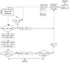
• If oi = zi, then do not change the weights as the patterns is already recognized correctly.
• If zi = 1 and oi = 0, then increase the weights of those neurons in the output layer which are connected to active elements in the intermediate layer j, hence wij(t + 1) = wij(t) + σ ∙ oj. In the next learning step, this increases the chance that zi = 1, so that the pattern is recognized correctly.
• If zi = 0 and oi = 1, then decrease the weights of those neurons in the output layer which are connected to active elements in the intermediate layer j, hence wij(t + 1) = wij(t) − σ ∙ oj. In the next learning step, this increases the chance that zi = 0, so that the pattern is recognized.
The value σ stands for the learning rate and determines the size of the weight change in each learning step. It normally assumes values in the range of [0; 1]. The value oj is the output of neuron j in the intermediate layer. The factor wij is the weight value with which oj is multiplied before the new value is fed into neuron i of the output layer. This type of learning process is called supervised learning.
Perceptron convergence theorem
Rosenblatt postulated that the learning algorithm as described above will converge within a limited period of time to the desired result provided that the neural network can represent the patterns in general. This gives no information on how long it will take for the ANN to learn to recognize all patterns. This depends on the structure of the network and how and in which order the patterns are fed into it. Besides, the initial values of the variable weight factors and also the values of the constant weight factors play an important role. The crucial aspect when applying perceptrons for pattern recognition is the question whether it can actually represent the problem at hand in general.
Problem of linear divisibility
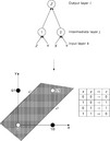
In 1969, Minsky and Pappert showed that perceptrons can learn not to recognize certain patterns. One of their examples was the parity determination and its special case, the XOR problem. This showed directly the weakness of perceptrons. The XOR function is one of 16 boolean operations with two variables. Its truth table is shown in Table 2.2. If the sum neti of the weighted inputs of the intermediate layer in the output element exceeds a threshold κ, the output element gives either a 0 or a 1. this is shown in Fig. 2.7 by the straight line, the so-called threshold line. it separates the area with neti > κ from the area with neti < κ. in order to represent the XOR problem with a single perceptron, the weights w1 and w2 must be determined in such a way that the points (0/0) and (1/1) are on one side of the threshold line and the points (0/1) and (1/0) on the other. It is apparent that this is not possible hence the XOR problem cannot be solved with a single perceptron. this type of function is called 'non-linearly separable' for which the perceptron does not converge.


2.7 XOR problem. (adapted from Schöneburg et al., 1990)
This problem can be overcome by introducing a second perceptron element which is connected with the first one with logical AND, as shown in Fig. 2.8. This leads to two threshold lines. The shaded area there is located in between the two threshold lines of the two perceptrons. It can therefore be separated from the surrounding area and the XOR problem can be solved. In principle, any non-linearly separable problem can be solved by logically connecting a sufficiently large number of perceptron elements. The resulting neural network structure can become very complicated and the required training time can be very long.
2.2.2 Adaline and madaline networks
Adaline and madaline networks are the result of further developments of the perceptron and the predecessor of today's most common ANN, the backpropagation network (see Section 2.3).
Adaline network
The adaptive linear neuron network was developed in the 1950s and is similar to the perceptron. Figure 2.9 shows its design. It consists of an input layer which is completely connected with the output layer via variable weights. The major difference to perceptron networks is the delta learning rule which is also an integral part of the backpropagation algorithm.

Similar to the perceptron, training is supervised, which means that input and output are known to the network during the training. In contrast to the perceptron algorithm, not the difference between desired output zi and actual output oi is calculated. Instead, the difference between the desired output zi and the activity ai of the neuron is determined. The actual output oi is a function of the activity ai (e.g. output oi = 1, if activity ai exceeds a threshold value κ). The delta learning rule is then as follows:
with δi = zi − ai, n = number of inputs (weights) of neuron i and σ = learning rate.
The prefix of the error and the value of the output of neuron j determine the direction and size of the weight change. A subsequent recall (another feeding into the network of the just trained pattern) leads to an error of 0 if the output function is chosen appropriately. Each adaline element learns (adjusts its weights) until its activity reaches the value of the desired output. Hence elements that already produce the correct output still adjust their weights as long as their activity is close to the threshold value. Thus, the distance between activity and threshold value is increased, which leads to a more stable state of the neural network as slight changes in the input pattern do not affect the output. In addition, once a pattern is trained, the neural network does not 'forget' the pattern as easily when other patterns are fed.
This behaviour resembles the biological basics as described in Section 2.1: a synapse which is activated often lowers its activation threshold, which leads to a quicker reaction. In the mathematical model, instead of lowering the threshold value, the weight factors are increased or decreased, which leads to the same result. Owing to this learning rule, the adaline network learns much quicker than a perceptron network. But it still faces the problem of non linearly-separable problems which is apparent by:
where n = number of input parameters and i = number of output neurons.
This equation system can be solved for at best n linearly independent (separable) input vectors. If more than n patterns are trained, only an approximate solution for each pattern can be found. In general, the capacity of adaline networks is in the range of n to 2n patterns.
Madaline network
The multiple adaptive linear neuron (madaline) network is an adaline network with an additional layer as shown in Fig. 2.10. Each element in the madaline layer is connected to exactly one madaline element via a constant weight factor of value 1. The output of the madaline element then depends on the difference between the number of active and passive neurons it is connected to and is hence always either + 1 or − 1. The learning rule of the adaline layer is similar to the learning rule as described in the previous section. If the classification of a madaline element is wrong, the weights of that element which activity is closest to 0 and which output has the wrong prefix are adjusted. Hence, the network can represent the input vectors internally in the hidden adaline layer and classify through its madaline elements. This separation also allows non-linearly separable problems to be solved, which is a prerequisite to tackle more complex tasks.

2.3 The backpropagation algorithm
In 1986, David E. Rumelhart, Geoffrey E. Hinton and Ronald J. Williams rediscovered a learning algorithm developed by Paul Werbos in 1974 (Werbos, 1974), the so-called backpropagation algorithm (Rumelhart et al., 1986). This was an improved madaline network type with a different structure and learning rule. The data are represented internally, the classification takes place in the output layer and learning is supervised. This algorithm makes it possible to solve non-linearly separable problems and, owing to the new learning rule, its learning speed is considerably higher than previous networks of, for example, the madaline type. Besides, much more complex network structures can be realized. Hence, backpropagation networks have a much higher capacity and can learn many more data sets than the nets described above. The direction of the information flow is feed-forward, the error of the output neurons is backpropagated through all layers back to the input neurons. This allows weights of neurons to be changed in the so-called hidden layers which are, in contrast to input and output layer, not visible from the outside. This is a new feature that did not previously exist.
2.3.1 Structure of the net
Figure 2.11 shows the structure of a neural net based on the backpropagation algorithm. In this typical example, each neuron is connected to all neurons of the previous and the subsequent layer. The capacity of the net (the number of data sets it can learn) is thus at a maximum. In the following, each layer is denoted with a letter, e.g. h, i, j, k, where layer j precedes layer i, hence being closer to the input layer. The weight factor wij therefore denotes the weight between neuron i in the current layer and the neuron j in the preceeding layer.

The input data are fed to the input layer j and multiplied with a variable weight factor wij. The sum of all inputs to a neuron of input layer j is then fed to the neurons of the first hidden layer i. The input function neti- of these neurons converts that input into a new value which is fed to the activation function Fi and subsequently to the output function fi of the neuron. In the following hidden layer (if existing), the outputs of the neurons of the preceding layer are multiplied with a variable weight whi and passed on to the next layer via input, activation and output functions neth, Fh and fh. This procedure is repeated until the output layer is reached. This information flow is shown in Fig. 2.12 for the fourth neuron of the first hidden layer in Fig. 2.11.

The neuron shown in Fig. 2.12 receives its input from all neurons of the preceding layer, multiplied with variable weight factors wij. This weighted input is then summed and passed on to the following layer via activation and output function. Most commonly used input functions are:
Most commonly used activation functions are:

The activation function must be derivable for reasons which are explained below. Any function meeting this requirement can be used. Normally, functions are applied that spread the data sets in order to simplify their classification. Most commonly used output functions are:
2.3.2 Learning rule
Backpropagation networks are trained with the generalized delta learning rule. The generalized form is derived here. Figure 2.13 depicts the prediction error of a simple neural network with only two weight factors depending on their respective values. It is the aim of the training to reach the minimum of the error area, in the ideal case zero. Then, the neural network would classify all fed data sets correctly. The error function is defined as

with W = weight vector of a layer and n = number of weights per layer.
The overall error of a given pattern is normally defined as the square difference between actual and desired output of the output layer:
Here, zi represents the desired output of neuron i and oi stands for the actual output. The factor 1/2 is introduced to later simplify to derive the function. A minimization of half the error implies the minimization of the error as a whole so this does have no negative effect.
The backpropagation algorithm is a gradient descent procedure. That means that the aim is minimizing the error by systematically changing the weight factors. The weight change in each training step by a fraction of the negative gradient of the error function E is given by:
we get the second factor in equation [2.9]
From equation [2.6] it follows, using the chain rule:
Insertion of [2.10] and [2.11] into [2.9] then leads [2.6] to:
From equation [2.12] it follows
For the second factor in [2.14] we get from [2.8]
For the output layer we get the first factor in [2.14], then to
Hence for the hidden layers we get:
This shows that the error of the neurons in the hidden layer i can be derived from the error of the neurons in the subsequent layer h which are connected with this neuron by weights whi.
For the neurons in the output layer we have:
For the hidden layers we get then:
In order to solve [2.18] and [2.19], the activation function must be derivable as mentioned above.
According to [2.6], we get the final form of the learning rule to adapt the weight factors as:
with the factor δ from [2.18] and [2.19]. This rule is also called the Hebb learning rule. The error of the output layer is therefore propagated back to the first hidden layer, which gives this algorithm its name: backpropagation.
2.3.3 Structure and capacity
Figure 2.11 shows all typical features of a neural network based on the backpropagation algorithm. The input layer is completely connected with all the neurons of the subsequent hidden layer and the neurons of the hidden layers themselves are also completely connected to the neurons of the subsequent layer. This not only increases the capacity of the neural net but also the prediction accuracy. If such a neural network is implemented into hardware, the failure of single connections between neurons does not then seriously affect the overall behaviour of the network as information is stored in a large number of connections (weights) between neurons. The last hidden layer is normally also fully connected to all neurons of the output layer.
The capacity of a neural network of this type depends mainly on the number of weights between the neurons. The more weights, the more information can be stored. For a given number of neurons, the maximum number N of weights can be calculated as follows: let ni be the number of input parameters, no the number of output parameters and k the overall number of neurons. For a network with two hidden layers, we get the optimum number of neurons s1 and s2 in each layer for N weight factors with:
Insertion of [2.22] into [2.21] leads to:
N reaches a peak value for ![]() = 0
= 0
After deriving [2.3], we get:
Example: For ni = 5 and no = 9 with k = 20, we get s1 = 8 and s2 = 12 with N = 244.
If a neural network with three hidden layers is to be optimized, two layers are considered as one and the calculation is carried out as described above. Then the neurons for the combined layers are distributed among the two layers in a similar way. In most cases, the capacity of a neural network with one or two hidden layers with 10–20 neurons each is sufficient to represent hundreds of data sets. Based on the author's experience, more than three hidden layers are never necessary. For the prediction of such a network to be accurate, a capacity which is adjusted to the complexity of the task at hand is crucial. If the capacity is too high or too low, the results of the prediction of the network for previously unknown input can be very imprecise.
2.3.4 Learning with the backpropagation algorithm
In this section, typical strategies to train a neural network using the backpropagation algorithm are explained and solutions for typical problems are discussed.
Initialization of the weight factors
At the beginning of the training stage, all weight factors wij are initialized with random values. Here, it is important to note that these values are truly random so that no symmetrical patterns occur. A symmetrical distribution of the weights would reduce the capacity of the network as several regions of the network would have identical weights. This cannot be changed during the training due to the learning rule derived above.
The delta learning rule according to Hebb is given by:
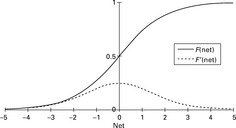
This implies that the weight change in a single learning step is increased with a greater error δi. This error is directly proportional to the derivative of the activation function F. The speed of the learning process can thus be increased by high values of the derivative of F. In most cases, the activation function F is the sigmoid function. Hence, all input values are transformed into the interval [0;1]. Values closely together and near zero are spread and thus separated for easier classification. The amount of spreading can be adjusted with the factor g, the so-called gain.
From the equation of the sigmoid function given by:
For g = 1, both functions are shown in Fig. 2.14. The value of the derivative assumes especially large values in the interval [–1;1] and reaches a maximum for net = 0. Hence, the weight factors are normally initialized with values within the interval [–1;1] or the interval [0;1].
The influence of the gain g on the function is shown in Fig. 2.15. A value of g > 1 results in a greater spreading of the functional values in [–1;1] the absolute value of the derivative is then very large. With values of g < 1, the functional values are closer to each other and the absolute value of the derivative is hence smaller. The weight factors are changed during the training but will nevertheless remain close to the interval [–1;1] normally in a range of [− 3;3].

Problems during training
Similar to all other gradient descent processes, one problem is that a local minimum is found which cannot be left by the algorithm. With increasing complexity of the network and hence a larger number of neurons and weight factors, the error area becomes more fissured. This in turn increases the probability of getting stuck in a local minimum. The following three cases are especially difficult to deal with.
Flat plateau
According to equation [2.18], the size of the weight change depends on the error δi. If this value was close to zero, the weight change becomes smaller and smaller and many learning steps are needed to leave such a minimum. In extreme cases, the local minimum cannot be left and the training process stops. Another difficulty is shown in Fig. 2.16. The gradient of the weight change for a flat plateau is close to zero as is the case for the absolute minimum. To distinguish one from the other is hence very difficult, if not impossible.

2.16 Flat plateau of the error function. (adapted from Schöneburg et al., 1990)
Steep crevices
As shown in Fig. 2.17, steep crevices of the error area can also be a severe problem. If the weight change is large, the algorithm results in a large step of the error function crossing the crevice. if the crevice is also steep on the other side, the error function will cause the algorithm to jump back to the side where it started from and so forth, it is very difficult to leave this vicious circle, requiring an adjustment of the learning rule during the training.

2.17 Steep crevices of the error function. (adapted from Schöneburg et al., 1990)
Missing a minimum
A very large weight change gradient when descending into a minimum (Fig. 2.18) may cause the algorithm to make a large step, thus crossing the sought minimum without having a chance to find it again. There are several ways to avoid or to overcome this problem. They are explained in the following section.

2.18 Missing a minimum of the error function. (adapted from Schöneburg et al., 1990)
Optimizing the training
Assuming an error landscape with large plateaus, many valleys and mountains, a sensible approach is to start with a large training rate, e.g. σ = 0.8, hence crossing and investigating the landscape in large steps to quickly find the region where the optimum is located. In order not to leave that area again, in later stages of the learning process, this value is gradually reduced to smaller values, e.g. σ = 0.1. in some cases, it is better to start with smaller values for the learning rate, that is a question of trial and error.
Momentum
In order to cross large plateaus (Fig. 2.16) quickly, the so-called momentum μ is another option. It is added to the delta learning rule which is then:
where Δwij(t) represents the weight change of the preceding learning step.
With the momentum factor, the general direction of the weight change is more likely to remain unchanged, thus avoiding local minima. Besides, when encountering steep crevices (Fig. 2.17), the learning speed decreases, hence large minima (at the bottom of the crevice) are more likely to be recognized. Small global minima can be missed though. Normally, μ values are in the range of 0.1 to 0.2.
Constant factor added to derivative
Another problem can arise when the sigmoid function is used as activation function. As was shown in Fig. 2.14, the maximum value of the derivate of the sigmoid function is F′(net) = 0.25. Hence, even if the difference between actual output and desired output is very large, resulting in a large (zi − Oi) value, the actual weight change is still comparatively small. The most simple method to overcome this problem is to add a constant factor c to the derivate F′(net), e.g. c = 0.1. This should only be considered at the beginning of the training as it can cause an unwanted prolongation of the training in later stages.
Weight decay
If the weight factors become too large, this can lead to oscillations and uncontrolled jumps across the error landscape. This can be avoided when the learning rule is modified as suggested by Paul Werbos as early as 1974 (Werbos, 1974). He introduced the weight decay d which leads to the following learning rule:
Here, a certain percentage of the previous weight value is deduced from the current weight change in order to keep the weight factors themselves from becoming too large. Normally, d is in the range of 0.005 to 0.03. This variant bears the risk of slowing down the learning process at an early stage as it may prevent the weight factors from becoming large enough to cross the error landscape quickly. It should therefore be used carefully and preferably in later stages of the training.
Data submission
Another important factor influencing the behaviour of the neural network during the training stage is the data submission method. For some applications, it makes sense to form groups of related data sets which are then fed into the network subsequently in those groups. For other applications where those groups cannot be formed, it is more sensible to feed them at random and not necessarily in the order in which they were gathered in experiments. If only a small network is to be used, the data sets can be divided into subgroups (at random) which are fed and trained subsequently. In this case, the neural network is initialized at the beginning, then the first subgroup is fed and trained and this trained network is then trained with the next data sets group, etc. It is apparent that it is difficult to define the optimal approach to train a neural network. The following examples are intended to illustrate typical training methods and their results.
2.3.5 Determination of suitable training parameters
After having calculated the optimum number of input and output nodes and the optimum network size, the following factors need to be determined:
According to the author's experience, it is sensible to start with a large learning rate (e.g. σ = 0.8). Hence, the weights are changed quickly and thus new patterns are learned and 'memorized' more easily. The learning rate is then gradually decreased until σ = 0.1. This consolidates the knowledge in later stages once it is acquired in the beginning. Momentum factors should be set in the range of 0.1 to 0.2. The truncation error determines when a training stage ends and the subsequent stage begins. Its value depends on the quality of the data submitted; typical values are in the range of 0.3 to 0.5 at the beginning (representing approximately 30–50 % overall prediction error) and 0.1 in the final training stage. The maximum number of generations is often set to 1000 at the beginning and then increased to values in the range of 3000–5000 in later stages.
Learning rate σ
The learning rate determines the weight change in each learning step. Large values lead to new knowledge being more quickly learned but also to existing knowledge being overwritten. At the beginning of the training stage, a large learning rate normally leads more quickly to the area where the optimum is located. If the learning rate is too large for too long, it is possible that the area of the optimum is completely missed. It is hence crucial to decrease it at the right time.
This is shown in Fig. 2.19. A large learning rate leads to a bumpy learning curve whereas smaller values of σ result in a smooth curve. It is noteworthy that the final result of the overall learning error (y-axis) is similar and not as dependent upon the learning rate as one would expect. A smooth course of the curve indicates that the neural network is in a stable state when the learning rate is small. An oscillating curve is a clear sign that the network alternates between meso-stable states. This implies that the predictions of such a network would not be very reliable.
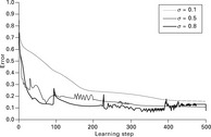
Figure 2.19 also shows that although the training itself is a gradient descent process, the overall error can increase during the training. Peaks indicate that new data sets are fed into the network that do not match previously acquired knowledge thus leading to large weight changes according to Hebb's learning rule.
Momentum factor
The momentum also affects the training course as is apparent in Fig. 2.20. A large momentum factor often leads quicker to a viable result as the direction of the weight change is maintained which allows, for example, large plateaus to be crossed more quickly. If the momentum factor is too high as in Fig. 2.21, the learning progress comes to a stop and the learning error oscillates.


Multi-stage training
Table 2.3 gives an overview of typical values for a training scenario consisting of five stages; while Fig. 2.22 shows the course of the learning error over time. The curves oscillate several times before the course becomes smooth and levels out at the end of the training. This is a typical behaviour of the network and due to changing training factors (e.g. learning rate) or when the network overcomes a local minimum.
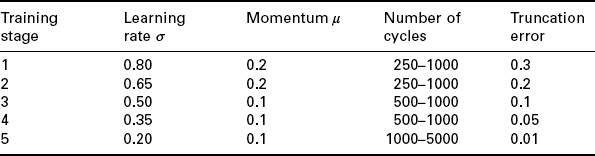
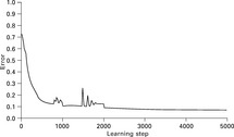
Figure 2.23 illustrates the gradual weight changes during the training. Each crossing point represents one weight factor. Different weight values are indicated by different grey values. Information flow in this example is from left (8 input nodes) to right (10 output nodes). The area in the upper left corner is therefore empty throughout the training as there are no weight factors. It is obvious that the weight changes at the beginning of the training are large and become smaller over time.

Typical example − texturing process
By texturizing synthetic yarns (POY − partially oriented yarns), they receive crimp and elasticity hence mechanical properties similar to staple fibre yarns (Fig. 2.24). The texturizing process comprises heating and cooling of the yarn, applying twist and winding up of the final product (DTY − draw textured yarn). The design of a texturizing machine is shown in Fig. 2.25.


Finding the optimum machine setting of a texturing machine is very difficult due to the large number of parameters that influence the process (e.g. yarn speed, heater temperatures, draft, POY, d/y-ratio) and hence the final yarn characteristics (e.g. tenacity, elongation, crimp). It has proven to be impossible to create a mathematical model that analytically describes the relations between machine settings and resulting yarn characteristics. Hence, when changing the yarn type or the yarn characteristics, a pilot test has to be carried out in order to determine the new machine settings.
In order to simplify this process, a neural network was employed to determine the relation between yarn characteristics and machine settings. Hence, it was possible to calculate the optimum machine setting for given yarn characteristics and also to predict the expected yarn characteristics depending on the machine settings (Veit, 1998; Veit et al., 1998).
Structure of the neural network
The neural network consisted of two hidden layers with 12 and 8 neurons each, similar to Fig. 2.11. The input function neti was the sum function, the activation function was the sigmoid function and the output function was linear.
Predicting the yarn characteristics depending on the machine setting
The network was trained with 36 data sets representing 36 different machine settings. Each set consisted of 15 machine parameters representing such factors as yarn speed, heater temperature, d/y-ratio and draft, and of 10 yarn parameters representing, for example, tenacity, elongation and crimp. From these sets, 35 data sets were used to actually train the network, and the remaining data set was used for the recall stage. This was repeated for all data sets. Hence, 36 neural networks were trained successively. A typical result is shown in Fig. 2.26. It is apparent that it was possible to train the neural network so that it could accurately predict the yarn characteristics from the respective machine settings.

Determining the optimum machine settings to achieve given yarn characteristics is much more difficult, as shown in Table 2.4. The prediction differs considerably from the expected result with which the yarn was actually produced. In Table 2.4, machine settings 12 and 18 and the resulting yarn profiles are shown which are similar to the desired yarn profile. It is apparent that these machine settings lead to a yarn profile similar to the one in question. The predicted machine setting resembles these settings and was therefore correct. The reason for this is typical for this kind of application: it is possible to achieve similar yarn profiles while using very different machine settings. During the training stage, the neural network normally learns to connect one of these possible settings with a certain yarn profile and hence makes a seemingly wrong prediction when fed this yarn profile. In fact, the predicted machine setting is one of many possibilities to achieve the same yarn characteristics.
Table 2.4
Comparison of predicted and actual machine settings to achieve certain yarn characteristics
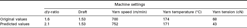

In contrast, a certain machine setting always leads to the same specific yarn profile. Hence, when predicting the yarn characteristics from the machine settings, this problem never occurs. The system does not only work in laboratory scale but has also been successfully employed in industry. Here, even the machine type and other parameters (e.g. describing the mechanical behaviour of the POY) not taken into account in the laboratory model, could be predicted correctly.
2.4 Counterpropagation
Despite their similar names, this algorithm is not related to the backpropagation algorithm. It was developed in the mid-1980s by Robert Hecht-Nielsen (1987, 1990) combining the earlier models devised by Teuvo Kohonen (1981) and Stephen Grossberg (1988). This algorithm is of the feed-forward type. The advantage of this neural network type is its learning speed, which is about 10–100 times higher than that of the backpropagation algorithm. Its drawback is the much lower capacity to represent patterns.
2.4.1 Network structure
The design of a counterpropagation network is shown in Fig. 2.27. The input data are normalized and the length of the input vector is set to 1. The Kohonen layer receives weighted input, and its weight factors are variable and can be trained. The length of the weight vector of each Kohonen neuron is set to 1. Each Kohonen element is connected to all elements of the input layer. The Kohonen neurons propagate their data to the Grossberg layer via variable weight factors where the length of the weight factor of each Grossberg element is again set to 1. All Grossberg neurons are connected to all Kohonen neurons.

2.4.2 Kohonen layer
The elements of the Kohonen layer are of the 'winner takes all' type: only that element with the greatest input becomes active whereas all other elements remain inactive. We have
with ![]() = weight vector of the Kohonen element.
= weight vector of the Kohonen element. ![]() and
and ![]() = input vector of the Kohonen layer. Hence:
= input vector of the Kohonen layer. Hence:
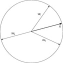
Figure 2.28 shows a graphic representation of weight vectors of Kohonen elements in two-dimensional space. The smaller the angle between weight vector and input vector the greater neti and thus ai. This implies that the Kohonen neuron which best resembles the input vector has the greatest activity. The input is thus classified according to its resemblance with the weight vectors of the Kohonen neurons.
2.4.3 Grossberg layer
For the Grossberg neurons, we have
Since there is only one Kohonen element active at any given time, we get:
The output of the Grossberg element i is equivalent to the weight factor between this element and the Kohonen element k.
2.4.4 Learning in the Kohonen layer
Learning in a Kohonen layer is non-supervised − also called 'discovering learning'. The output vector must therefore not be known to the Kohonen elements. This is one of the major differences to the backpropagation algorithm. According to the 'winner takes all' rule, we have:
Figure 2.29 shows a two-dimensional graphic representation of the learning process of the Kohonen neurons. The learning rate σ is normally smaller than 1 in the beginning and is subsequently decreased until it reaches the value σ = 0. The length of the weight vector can decrease during the training. The smaller the distance between weight vector and respective input vector, the smaller their difference in length. Hence, at the end of the training, all weight vectors have again a length of 1.
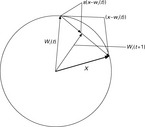
The weight vectors of the Kohonen elements move towards those input vectors which they resemble best. Hence, all weight vectors of the Kohonen neurons change. The change increases with the activity of the Kohonen elements which in turn increases the more the respective weight vector resembles the particular input vector. At the end of the training stage, the weight vectors of the Kohonen elements are located roughly in the middle of those input vectors which they represent best. This implies that the Kohonen layer mirrors all learned input vectors not only in terms of location but also statistically. Hence, in areas with many input vectors, the number of Kohonen vectors is also large. With n = number of Kohonen elements, the probability that a certain Kohonen neuron becomes active during a learning step becomes 1/n. If n equals the number of input vectors, the training is completed after only one step. In this case, each input vector would exactly be represented by one weight vector.
2.4.5 Initializing the weight factors of the Kohonen layer
Normally, the weights of the Kohonen elements are initialized with small, randomly chosen values with the norm 1. A typical problem arising then is the uneven distribution of weight and input vectors that is ideally identical. As shown in the example in Fig. 2.30, only a few weight vectors represent input vectors; several weight vectors represent nothing. It is therefore an absolute necessity to distribute weight vectors and input vectors evenly. Normally, though, the distribution of the input vectors is unknown or difficult to determine. Hence, several methods were developed to overcome this problem. They are described in the following sections.

Convex combination
All weight vectors are initialized with the unit vector:

The input vectors are then fed into the vector according to
In the beginning, the value α is close to zero and increased gradually during the training stage until α = 1. This leads to weight vectors being dragged along with the input vectors, thus resulting in even weight and input vector distributions. The advantage of this method is the good representation of the input vectors by the weight vectors. The major drawback is the time needed to train all input patterns as they change during the course of the training.
Random noise
A random noise can be added to the input vectors. Hence we get
Thus in principle, all Kohonen elements can win, even those which resemble the input vector less than others. The input vectors themselves do not change during the training. This method is even more time-consuming than the convex combination. But all weight vectors partake in the learning process which can be advantageous and normally avoids weight vectors left in the void without representing anything.
Radius
All weight vectors within a given radius around the input vector partake in the learning process. If the radius is sufficiently large, all Kohonen elements can learn. The radius value decreases during the training until it reaches zero, so that finally the only Kohonen element that learns is the one which resembles the input vector best. This leads to a good representation of the input vectors but is very time-consuming.
2.4.6 Interpolative mode in the Kohonen layer
The output of the Kohonen layer normally consists of the output of the winning element. If not only one but several Kohonen elements actually win, then we have
The norm of the output of the Kohonen layer is still equal to one. This value is distributed among all winning Kohonen elements according to their activity, hence
The learning rule of the Kohonen elements can then be written as
The smaller the distance between ![]() and
and ![]() at point in time t, the greater oi and hence the more the weights are adjusted at point in time t + 1.
at point in time t, the greater oi and hence the more the weights are adjusted at point in time t + 1.
2.4.7 Training of the Grossberg layer
The elements of the Grosberg layer learn supervised as the desired output is known. The learning rule is then:
with zi = desired output of Grossberg elements i and oj = output of Kohonen element j. It is assumed that only one Kohonen element is active at any given time, hence there is only one oj ≠ 0.
For σ = 1, the weight factors wij of the Grossberg layer to this Kohonen element j become equal to the desired output zi. Normally, σ assumes very small values (e.g. σ = 0.1) which are gradually increased until σ = 1.
At the end of the training stage, a certain group of input vectors is represented by one Kohonen element. The weight vector of this Kohonen element connecting it to the Grossberg layer represents those output vectors, to which the input vectors correspond.
2.4.8 Network structure
The typical structure of a counterpropagation network is shown in Fig. 2.31. Input and output layers are divided into two parts. Hence, there are virtually two input and two output layers that are identical. The input is fed into layers x and y; the resulting output is then X' and Y'. The name counterpropagation relates to another graphical representation of the network as shown in Fig. 2.32. If the vectors x and y are doubled (X', Y') and drawn one on each side of the Kohonen layer, the information flow is inward bound, thus giving this network type its name.

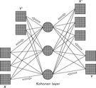
2.32 Another graphical representation of a counterpropagation network. (adapted from Schöneburg et al., 1990)
The training of this network is auto-associative. This means that the vectors X and Y are associated with themselves. Hence, if X and Y are fed into the network during the recall, the network will produce X′ and Y′ as output. If only the vector X is fed into the network and all values of vector Y are set to zero, the output will normally still be X' and Y'. The network is therefore able to learn the relation between X and Y' and also between its inverse function, Y and X'. This is very useful for pattern recognition applications as it allows an easy reversal of the contrast of a picture. In general, this type of neural network is especially suitable for all classification problems where groups of data sets need to be clustered and only the number of clusters is known but not their exact boundaries. Typical applications in textiles are pattern recognition or classification of faults in fabrics.
2.5 Other types of neural networks
Apart from the previously mentioned network types, there are also a range of other kinds of networks suitable for special applications.
2.5.1 Hopfield networks
This network is of the feedback type. In the first step, input is fed into the network which generates output. This output is then fed into the network as new input. This process is repeated until all patterns reproduce themselves. This is a stable state which can be defined using an energy function. This kind of network can be used to recognize patterns with a random noise. Another interesting feature is the ability of this network type to eradicate learned patterns from its memory. This can be helpful when training patterns over a large period of time when the first patterns should be deleted and replaced by later ones.
2.5.2 Simulated annealing
This is another interesting type of network to determine global minima. It works in a totally different way from backpropagation and counterpropagation algorithms, but is nevertheless considered an ANN. During the training stage, it is possible to leave local minima, thus deteriorating the quality of the output. Hence, it is possible to find the global minimum which is more difficult with Hopfield networks. There are a number of other types of neural networks, but they are currently not used to solve technical problems in textile production.
2.6 Applications of neural networks to textile technology
In recent years, neural networks have been used successfully to solve numerical problems for a wide range of applications. These include pattern recognition (Wei et al., 2010), language recognition (Ververidis and Kotropoulos, 2006), material inspection (Su et al., 2008), machine optimization (Veit, 1999), the prediction of product performance (Liu and Qu, 2008) and many more. In textile technology, there have also been a wide range of successful applications as the number of published papers shows (Fig. 2.33). In the following sections, typical examples for such applications are briefly described. They all use the backpropagation algorithm unless otherwise stated. Many more papers have been published in recent years, but often with questionable results as verifiable data were not given or unscientific evaluation methods were used. These are hence not cited in this section.

2.33 Number of published papers on neural network applications in textiles (Anon, 2011).
2.6.1 Pattern recognition
A typical example for this kind of application is the detection of trash particles in fibre webs. The influence of the machine settings in the cleaning room on the cleaning efficiency was analysed by Veit et al. (1996a, 1996b). Fibre samples were taken before and after each cleaner and analysed applying digital image processing in connection with a neural network. The neural net was used to classify the trash particles (e.g. neps, seed coat fragments, leaf and stem fragments). Figure 2.34 shows the digital image of a fibre web.

2.34 Digital image of a fibre web (Veit et al., 1996b).
The backpropagation neural network consisted of five neurons in the output layer, each representing one kind of trash particle. Three hidden layers were used with 10, 15 and 20 nodes, the input layer consisted of 10 nodes each representing parameters that describe the trash particles. In the initial stage, the neural net was trained with 1500 data sets, each describing a typical trash particle with regard to size, circumference, shape, etc. Prediction accuracy after the training stage was close to 95%. Then, particle data sets unknown to the network were fed into the system and the particles were classified with an accuracy of approximately 85%. The comparison of manually classified particles and the results of the neural network analyser showed a high degree of consistency, as can be seen in Fig. 2.35.

2.35 Comparison of classification result for neps: manual vs. digital image processing with neural network analyser (Veit et al., 1996b).
It was very difficult to distinguish between seed coat fragments, leaf particles and stem particles as these kinds of particle appeared very much alike to the system. In order to further improve the accuracy, a fuzzy algorithm was implemented in the output layer of the neural network. This led to a significantly higher accuracy as even when two output neurons showed a similar activity, a fuzzy rule could help to determine the actual kind of particle.
The major advantage of this neuro-fuzzy system compared with conventional methods was the classification time which was only a matter of seconds for several hundred data sets gathered when screening one digital image of a fibre web. Conventional systems (e.g. nearest neighbour classification) took several minutes with a considerably lower accuracy (e.g. approx. 75% for nearest-neighbour algorithm).
2.6.2 Draw frame
Farooq and Cherif (2008) developed a system to determine the levelling action point (LAP) of an auto-levelling draw frame. Input parameters comprised, for example, feeding and delivery speed, break and main draft gauge. Several different network structures, all based on the backpropagation algorithm, were used. As Fig. 2.36 shows, the prediction accuracy was very high and reached 98% on average in this example. Here, two hidden layers with 12 and 10 neurons each were used. The maximum deviation between predicted and actual optimum LAP values does never exceed 3 mm which falls within the range of negligible differences when determining the LAP, as practice trials showed.
2.36 Comparison of predicted and actual LAP. (adapted from Farooq and Cherif, 2008)
2.6.3 Hairiness of worsted yarns
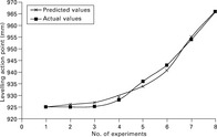
Wang et al. (2009) developed a prediction model for the hairiness of worsted yarns. They used one hidden layer with only one hidden node, a learning rate of σ = 0.3 and a momentum factor of μ = 0.9. A sensitivity analysis (see Section 2.7.1) showed that several of the originally used input parameters did not have a decisive effect on the hairiness (Fig. 2.37). Hence, only yarn twist, ring size, hauteur, mean fibre diameter, yarn count, short fibre proportion and spindle speed were needed to predict the expected yarn hairiness very accurately as can be seen in Fig. 2.38.
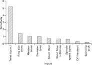
2.37 Typical sensitivity values. (adapted from Wang et al., 2009)

2.38 Comparison of predicted and actual hairiness values. (adapted from Wang et al., 2009)
2.6.4 Draw-winding process
Draw-winding is an important process to produce high tenacity yarns, mainly from polyester and polyamide. The principle is shown in Fig. 2.39. Small-and medium-sized enterprises often apply this process but rely heavily on the expert knowledge of mostly senior engineers. When they retire, their knowledge is often lost. This led to the development of a system based on a neural network that was able to determine the machine settings to achieve certain yarn profiles and vice versa (Ramakers, 2006). Each of the 50 data sets used consisted of parameters describing the machine set-up (e.g. temperature of godets, draft ratios) and others representing the yarn profile (e.g. yarn fineness, tenacity, shrinkage). Figure 2.40 shows the basic approach to training a neural network with these data sets.
![]()
2.39 Basic design of the draw-winding process. (adapted from Ramakers, 2006)

2.40 Basic approach to training the neural network. (adapted from Ramakers, 2006)
In this case, the first results showed that the neural network was not able to learn the relation between yarn profiles and machine settings. Thus, a design of experiments (DoE) approach was applied where the machine settings were varied in a very structured way hence covering a much wider range of the parameter values. This greatly improved the accuracy of the prediction, as is shown in Fig. 2.41. The average prediction error was below 3%.

2.41 Comparison between predicted and actual yarn tenacity in the draw-winding process. (adapted from Ramakers, 2006)
2.6.5 Weaving process
In recent years, the machine speed in the weaving process has been increased considerably. This has led to ever-greater difficulties to ensure a high fabric quality. Especially after a machine stop, the so-called stop marks in the fabric (caused by an uneven spacing between weft threads, Fig. 2.42) are a fault which is no longer acceptable owing to increased market requirements. Hence, a mathematical model was developed by Strauf, Amabile and Gries (2005) describing the relations between machine settings, fabric properties and stop mark characteristics.
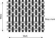
2.42 Stop mark in a fabric. (adapted from Strauf Amabile and Gries, 2005)
Table 2.5 gives an overview of typical parameters having an influence on the characteristics of a stop mark. It is apparent that there are many different parameters to be taken into account which makes an analytical description of the relations almost impossible. Hence, a neural network was used and trained with data sets representing typical machine settings, fabric properties and resulting stop mark characteristics. This was used to determine an optimum machine setting in order to minimize the stop mark hence minimizing the effect of a machine stop on the fabric quality. Table 2.6 shows a comparison of predicted and actual machine settings during the training. Figure 2.43 shows the predicted characteristics of a stop mark (here: spacing between weft threads after a machine stop) and the measured data. Since the system apparently works, it is now used in industry by weaving machine manufacturers.


2.43 Predicted and actual stop mark characteristics. (adapted from Strauf Amabile and Gries, 2005)
2.6.6 Yarn breakage rate during weaving
Yao et al. (2005) published a paper on the prediction of warp breakage rate using a backpropagation network. Input values included size add-on, abrasion resistance, breaking strength and hairiness. The authors claim to have reached a prediction accuracy for the number of yarn breaks close to 90%, but no verifiable data base is provided. Bo (2010) used a similar approach, but again no verifiable data were presented and the used input values were not specified. In general, according to the author's experience, it is very difficult to predict breakage rates as there is a strong influence of non-measurable factors which normally cannot be neglected.
2.6.7 Yarn shrinkage
Lin (2007) developed a system to predict the shrinkage of weft and warp yarns depending on the cover factors of warp, weft and fabric as input. This is a very difficult problem as shrinkage strongly depends on the deformation of the yarns and various other factors that are very hard to keep constant. He used one hidden layer with 16 neurons, a learning rate of σ = 0.9 and a momentum factor μ = 0.9 which are relatively high values. Lin trained the network with 13 data sets and used 13 others for the recall stage. The results are shown in Fig. 2.44. The value for R2 = 0.8723 in this example is high and indicates that applying a neural network is a sensible approach to tackle this difficult problem.

2.44 Comparison between measured and predicted warp shrinkage. (adapted from Lin, 2007)
2.6.8 Spirality of cotton fabrics
Murrells et al. (2009) used a neural network to predict the spirality of fully relaxed single jersey fabrics made of 100% cotton. As input factors, they used twist liveliness, yarn type, yarn linear density, fabric tightness factor, number of feeders, rotational direction, gauge of the knitting machine and dyeing method. After determining the most important factors to be used as input values, they trained a feed-forward network (probably backpropagation) with one hidden layer and a different number of neurons with 40 data sets, 26 were later used for the recall. The results were very good, as can be seen in Fig. 2.45. The correlation coefficient was R = 0.976 compared to R = 0.970 for a multiple regression model.
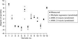
2.45 Predicted and measured degree of spirality for eight input factors. (adapted from Murrells et al., 2009)
2.6.9 Textile fabric appearance
Cherkassky and Weinberg (2010a) used a probabilistic neural network approach (related to Kohonen nets) to determine the grades of knitted fabric appearance. This is a typical classification problem for which this type of neural network is perfectly suited. Photographs were taken from the samples and analysed. The input values of the network were the calculated fabric brightness, the average number of pills and fuzzy and the average and standard deviation for all captured profiles. The output layer consisted of five nodes with each representing a different grade. As Fig. 2.46 shows, the predicted grades coincide very well with the grades given by experts (Cherkassky and Weinberg, 2010b). Taking into account that the expert grades may also not all be correct, the achieved results are excellent.

2.46 Comparison of predicted and actual grades for the knitted fabrics. (adapted from Cherkassky, 2010b)
Another paper dealing with this subject focusing on polar fleece fabrics was published by Xin et al. (2010). Chen and Zhang (1999) applied a backpropagation network for fibre content analysis. They developed a system that could distinguish between yak and cashmere hair based on microscopic images that reached a classification accuracy of 92%. A similar system was published by Shi and Yu (2008). It was used to identify animal fibres, namely wool and cashmere, where it reached a prediction accuracy exceeding 90%. The network used was very small with only one hidden layer containing five nodes. This shows that ANNs do not need to be complicated to solve complex problems.
2.6.10 Fabric inspection
Yuen et al. (2009) used the backpropagation algorithm for the automatic defect detection, namely for evaluating fabric stitches and seams. Pictures of the fabrics were taken and nine characteristic parameters were used as input values. Since the value ranges differ, a data preprocessing method was required which transforms all input values into a similar range. The output layer consisted of only two neurons. They could assume only binary values leading to four different output patterns, 00, 10, 01, 11, of which three were used to associate the image with one of the three classes: 'seams without defects', 'seams with pleated defects' and 'seams with pucking defects'. One hidden layer was used with 10 neurons. The training set consisted of 22 samples for each class and an additional 10 samples were used in the recall stage. Although the output nodes did not always lead to values of 0 or 1 respectively (Table 2.7), the rounded results were always 100% correct. This example shows that the backpropagation algorithm is also very suitable to solve classification problems.
Table 2.7
Comparison of calculated outputs and actual values

Source: adapted and shortened from Wang et al., 2009.
A similar approach to detect local textile defects using a neural network was published by Kumar (2003). It gives a comprehensive overview of feature detection from photographs aimed at training a neural network and is therefore recommended reading for anyone interested in fabric inspection. Other papers on this subject worth reading include those of Liu and Qu (2008), Yin et al. (2009) and Chandra et al. (2010). Papers by Pan et al. (2011) and by Kuo et al. (2010) deal with woven fabric pattern recognition in a similar way. Both papers provide extensive information on the methods applied.
2.6.11 Design of airbag fabrics
Behera and Goyal (2009) applied a backpropagation network to predict the performance parameters for airbag fabrics. The input parameters include fabric areal density, ends and picks per inch, warp and weft yarn count, strength and elongation. The results for the different output parameters are shown in Table 2.8. The values were calculated as the mean of the results of five samples that were used in the recall stage.
Table 2.8
Average error for different output parameters

Source: adapted from Behera and Goyal, 2009.
It is apparent that the average error strongly differs for different parameters: air permeability is very hard to predict whereas the tensile strength in the warp and weft directions is calculated very accurately. Apart from physical explanations for this problem, another reason could be the application of a single neural network to predict all parameters at once. In cases such as this, the use of separate neural networks where each predicts only one parameter normally improves the overall result. This is because, firstly, each neural network structure could then be tailored for each parameter and, secondly, that the relations between input and output values do not affect each other during training.
2.6.12 Thermal resistance and thermal conductivity of textile fabrics
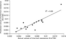
Kothari and Bhattacharjee (2007) applied two different neural networks to predict the steady-state thermal resistance and the maximum instantaneous heat transfer Qmax of woven fabrics. The input parameters included weave type, weft and warp count, weft and warp density. The neural network had two hidden layers. At first, for each output parameter, a separate network containing a small number of neurons in each hidden layer was trained and the prediction compared with the measured values. Then, a network consisting of two hidden layers with a higher number of nodes was used to predict both output values simultaneously. This increased the mean error from 8.6% to 10.4% (see also Section 2.6.1). Figures 2.47 and 2.48 show the results for both output values for both cases. Both thermal resistance and heat transfer could be predicted with sufficient accuracy with thermal resistance showing better results.

2.47 Comparison of calculated thermal resistance and actual values (one neural net). (adapted from Kothari and Bhattacharjee, 2007)
2.48 Comparison of calculated heat transfer and actual values (two neural nets). (adapted from Kothari and Bhattacharjee, 2007)
Majumdar (2011) describes a model based on the backpropagation algorithm to predict the thermal conductivity of knitted fabrics made of cotton-bamboo yarns. As input parameters, he used the structure, the thickness and the area weight of the knitted fabric, the yarn count and the bamboo fibre content. The fabric structures were encoded using − 1, 0 and + 1 to represent the three different kinds. One hidden layer with three nodes was sufficient to accurately predict the thermal conductivity of the fabrics. A trend analysis showed the influence of each input parameter on the conductivity value.
2.6.13 Protective textiles
Ramaiah et al. (2010) investigated the possibility to predict the performance of ballistic fabrics made of Kevlar 29 using their material properties as inputs. In order to avoid overfitting, great care was put on the selection of suitable data sets representing the whole range of parameter values. The input parameters included the specific modulus of the fibre and its tenacity, the fibre density, warp and weft yarn count and impact velocity of the projectile. The output parameters were penetration depth and dissipated energy by the fabric. One hidden layer was sufficient to give excellent results as can be seen in Figs 2.49 and 2.50. Only one network was used to predict both values simultaneously. The achieved results can be used to design and develop new ballistic protection fabrics without having to carry out time-consuming and costly destructive tests.

2.49 Comparison of predicted and measured values for penetration depth. (adapted from Ramaiah et al., 2010)

2.50 Comparison of predicted and measured values for dissipated energy. (adapted from Ramaiah et al., 2010)
2.6.14 Emotion-based textile indexing
A truly innovative application of neural networks in textiles was published by Kim et al. (2007). They used a neural network to predict the emotional response of humans on specific textile patterns. At first, they developed a system using wavelet transformation techniques to extract special features out of textile patterns. Then, they trained a network with this information to relate it to descriptive, emotional terms such as dynamic, modern and casual. A comparison of the calculated emotional response on a wide range of patterns with the actual answers of test persons showed an accuracy of about 90%. This example shows the wide range of applications of neural networks.
2.6.15 Smart carpet
Another application was developed by Infineon Technologies, Germany. A self-organizing, fault-tolerant microcontroller network based on RFID technology (radio frequency identification) was integrated into a carpet. Through connected sensor elements, it is possible, for example, to detect the position of a person on the carpet or to measure the temperature on a certain spot. Each sensor node or neuron is connected to its four nearest neighbours to which it can pass on information. Upon initializing the system, each neuron determines its position relative to the others. In case of a sensor failure, the system still works as this neuron is then disregarded by its neighbours. Hence, the carpet can be cut into pieces without impairing its functionality (Anon., 2003).
2.6.16 Other applications
Other interesting papers on the application of neural networks in textiles in a broader sense that are not described in detail here include one on the stationary solution of the geometrical shape of the ring-spinning balloon in zero air drag by Tran et al. (2010) and another on the modelling of an industrial plant for the biological treatment of textile wastewaters by Molga and Cherbanski (2006).
2.7 Practical advice in applying neural networks
In this section, advice is given on how to tackle typical problems that are often encountered when trying to apply a neural network.
2.7.1 Significance of input parameters
For many applications, the number of possible input parameters is too huge for practical use. Therefore, it is essential to determine the most important input parameters before actually starting the training stage. In addition, connected parameters should be determined and reduced to the one parameter that can be measured or set easiest by eliminating all the others. Then, all remaining parameters should be analysed with regard to their significance on the output values. A simple method to achieve this was published by Wang et al. (2009). They calculate a so-called sensitivity value Sk for each input parameter by varying its value around its mean value and observing the change of the calculated output for all patterns with all weight factors unchanged according to:
where p is the pattern number, o is the number of network outputs, k denotes the input parameter, yip stands for the trained output and ![]() represents the variance of the input perturbation. This simple method quickly shows which parameters may have a significant influence on the output parameters and should therefore considered when training the network. A typical example, taken from Wang et al. (2009), is shown in Fig. 2.37. It is apparent that the input values CVH and CVD as well as spinning draft can be neglected without affecting the prediction too much.
represents the variance of the input perturbation. This simple method quickly shows which parameters may have a significant influence on the output parameters and should therefore considered when training the network. A typical example, taken from Wang et al. (2009), is shown in Fig. 2.37. It is apparent that the input values CVH and CVD as well as spinning draft can be neglected without affecting the prediction too much.
2.7.2 Network structure and size
The performance of a neural network during the training stage can be judged by the size of the summed difference between calculated and desired output. Since the desired output is known to the network, this overall training error is normally less than 10%. Whether a neural network has actually recognized the relations between input and output parameters or just learned 'by heart' to relate these parameters can be determined only in the so-called recall stage (see Fig. 2.3). If the network has actually learned the relations, it is called well generalized. If the network is not sufficiently complex (e.g. too low number of neurons in a too low number of hidden layers), despite a good training result, the recall accuracy will be poor (below 50%). The network is then called underfitted. A more common problem is an overfitted network. In this case, the network structure is too complex, thus detecting relations between input and output parameters that are caused by noise in the data rather than by actual and sensible differences in the respective values. A sensitivity test as described above can help to reveal an overfitting network. However, only a test with real data shows whether a neural network is well generalized, hence leading to reliable and accurate output or not. The optimum network size for one or two hidden layers can be calculated as described in Section 2.3.3.
2.7.3 Database
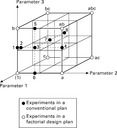
In many cases, the available database is taken from production data sheets and hence has often not been collected systematically. This can lead to training data sets that overrepresent certain regions of the parameter space and completely lack data sets in others. This can be avoided with data sets that are gathered using experimental design (factorial design) thus ensuring that boundary values are taken into account during the training stage (Fig. 2.51). As it is much easier for a neural network to interpolate than to extrapolate, this greatly improves the performance of a neural network since extreme values for each parameter are part of the training set.
2.7.4 Recall stage
An important question which has to be answered before beginning training is the proportion of data sets which has to be set aside during the training to be used later in the recall stage. In general, a minimum of 10% of the available data sets should not be used during training. if these data sets are then fed into the network during the recall, a vast majority of the predictions should be sufficiently accurate in order to have a degree of certainty that the network is well generalized. if the number of data sets is very small, a different approach is to use all but one of the data sets for the training and to feed the remaining in the recall stage. This has to be repeated with different nets (same structure) for all patterns (see Fig. 2.52). Hence it will be apparent whether the neural network has learned the relations between input and output and can thus predict each output correctly.

A commonly made error which can be found in many papers not cited here is to compare the calculated with the actual output and determine a relative error as shown in Table 2.9. At first glance one would think that the predictions of the neural network are very precise. in reality, it is obvious that the neural network has learned to relate input value 2 with the output value. The deviation of the predicted output values is in fact the same as the deviation of the actual output values. This result does not prove that the network has actually recognized any relation. This problem is related to the one described in Section 2.7.3 and could have been solved using factorial design to have a representative database.

2.8 Summary
As the examples described show, neural networks can be a powerful tool to solve a wide range of problems. Their application offers a wide range of advantages compared to other models when solving numerical problems. The main advantage of these systems is there commercial availability which allows the user to concentrate on providing data sets rather than having to design a new computer model.
But there are also a number of risks of which the user should be aware. A major drawback is the fact that it is not possible to understand in a mathematical sense the relations between input and output data which the network has found. A test run with patterns that are unknown to the network can give an indication but no certainty whether the predictions of the trained network will be accurate. A famous example of how not to train a neural network was carried out in the USA in the 1960s. A system was devised to recognize armoured vehicles even when camouflaged. The neural network was trained with photographs of landscape with and without vehicles. in the lab-recall stage, the prediction accuracy was 100%. A practice trial ended in disaster as the system failed completely. All photographs with vehicles had been taken in sunshine, all the others with overcast sky. The system had learned to perfectly distinguish between different weather conditions but not to detect camouflaged vehicles. Hence, all prospective users are strongly advised to always test their systems in practice and not only in laboratory scale before relying on the predictions and making any promises to customers.
2.9 Web references for software tools
There is a wide range of software tools and general information on the world wide web. The following links are a selection of useful websites.
Neural network software
http://www.kdnuggets.com/software/classification-neural.html
http://www.simtel.net/category/Neural-Network-Programs/207.html
http://www.dmoz.org/Computers/Artificial_Intelligence/Neural_Networks/Software/
Free neural network software
http://www.membrain-nn.de/main_en.htm
http://sourceforge.net/projects/joone/index.html
http://www.ra.cs.uni-tuebingen.de/software/JavaNNS/welcome_e.html
http://axel-arnold.de/index.php?id=68&L=2
Commercial neural network software
http://www.crgraph.de/index.html
http://www.mathworks.com/products/neuralnet/
http://www.neurosolutions.com/
Other sources
A list of publications dealing with the application of neural networks is given here:http://synapse.cs.byu.edu/publications.php
One of the early standard books about neural networks covering a wide range of net types and theoretical aspects is available online here:http://page.mi.fu-berlin.de/rojas/neural/
A forum for forecasting applications using neural networks can be found here:http://www.neural-forecasting.com/
2.10 References and further reading
Anon. Magic carpet ride. Expert Systems. 2003; 20(5):312.
Anon. Literature survey, 2011. http://www.engineeringvillage2.com [[accessed 17 May 2011].].
Behera, B.K., Goyal, Y. Artificial neural network system for the design of airbag fabrics. Textile Research Journal. 2009; 39(1):45–55.
Bo, Z., The prediction of warp breakage rate of weaving by considering sized yarn quality using artificial eural network theory. 2010 International Conference on Computer Design and Applications, ICCDA 2010, 2010:V2526–V2529. [vol. 2].
Chandra, J.K., Banerjee, P.K., Datta, A.K. Model modification and prediction of mechanical behavior of fabrics in uniaxial tension. Journal of the Textile Institute. 2010; 101(8):699–706.
Chen, C.H., Zhang, X., Using neural networks for fiber content analysis. Proceedings of the International Joint Conference on Neural Networks, 1999:3913–3916. [6].
Cherkassky, A., Weinberg, A. Objective evaluation of textile fabric appearance part 1: Basic principles, protrusion detection, and parameterization. Textile Research Journal. 2010; 80(3):226–235.
Cherkassky, A., Weinberg, A. Objective evaluation of textile fabric appearance part 2: SET Opti-grade tester, grading algorithms, and testing. Textile Research Journal. 2010; 80(2):135–144.
Farooq, A., Cherif, C. Use of artificial neural networks for determining the leveling action point at the auto-leveling draw frame. Textile Research Journal. 2008; 78(6):502–509.
Grossberg, S. Nonlinear neural networks: principles, mechanisms, and architectures. Neural Networks, vol.. 17-61, 1988.
Halleb, N. Model modification and prediction of mechanical behaviour of fabrics in uniaxial tension. Journal of the Textile Institute. 2010; 101(8):707–715.
Hebb, D.The Organization of Behavior: A Neuropsychological Theory. Lawrence Erlbaum Assoc Inc, 2002. [(new edition of book published in 1949).].
Hecht-Nielsen, R. Counterprogagation networks. Applied Optics. 1987; 26(23):4979–4984.
Hecht-Nielsen, R. Neurocomputing. Reading, MA: Addison-Wesley; 1990.
Kim, N.Y., Shin, Y., Kim, E.Y., Emotion-based textile indexing using neural networks. Proceedings of the International Symposium on Consumer Electronics, ISCE, 2007.
Kohonen, T., Automatic formation of topological maps of patterns in a self-organizing system. Proceedings of 2SCIA, Scand. Conf. on Image Analysis. Helsinki, Finland, 1981:214–220.
Kothari, V.K., Bhattacharjee, D. A neural network system for prediction of thermal resistance of textile fabrics. Textile Research Journal. 2007; 77(1):4–12.
Kumar, A. Neural network based detection of local textile defects. Pattern Recognition. 2003; 36(7):1645–1659.
Kuo, C.-F.J., Shih, C.-Y., Ho, C.-E., Peng, K.-C. Application of computer vision in the automatic identification and classification of woven fabric weave patterns. Textile Research Journal. 2010; 80(20):2144–2157.
Lin, J.-J. Prediction of yarn shrinkage using neural nets. Textile Research Journal. 2007; 77(5):336–342.
Liu, J., Zuo, B., Zeng, X., Vroman, P., Rabenasolo, B. Nonwoven uniformity identification using wavelet texture analysis and LVQ neural network. Expert Systems with Applications. 2010; 37(3):2241–2246.
Liu, S.-G., Qu, P.-G., Inspection of fabric defects based on wavelet Analysis and BP neural network. Proceedings of the 2008 International Conference on Wavelet Analysis and Pattern Recognition, ICWAPR, 2008:232–236. [vol. 1].
Majumdar, A. Modelling of thermal conductivity of knitted fabrics made of cotton-bamboo yarns using artificial neural network. Journal of the Textile Institute. 2011; 102(9):752–762.
McCulloch, W., Pitts, W. A heterarchy of values determined by the topology of nervous nets. Bulletin of Mathematical Biophysics. 1945; 7:89–93.
Minsky, M., Papert, S. Perceptrons. Cambridge: MIT Press; 1969.
Molga, E., Cherban ski, R. Modelling of an industrial full-scale plant for biological treatment of textile wastewaters: Application of neural networks. American Chemical Society. 2006; 45(3):1039–1046.
Murrells, C.M., Tao, X.M., Xu, B.G., Cheng, K.P.S. An artificial neural network model for the prediction of spirality of fully relaxed single jersey fabrics. Textile Research Journal. 2009; 79(3):227–234.
Pan, R., Gao, W., Liu, J., Wang, H. Automatic recognition of woven fabric based in image processing and BP neural network. Journal of the Textile Institute. 2011; 102(1):19–30.
Ramaiah, G.B., Chennaiah, R.Y., Satyanarayanarao, G.K. Investigation and modeling on protective textiles using artificial neural networks for defense applications. Materials Science and Engineering B. 2010; 168(1):100–105.
Ramakers, R., Systematical method for development of sensor-based quality monitoring of man-made fiber processing − drawing, winding, texturing. Proceedings of the International Man-Made Fibres Congress. Dornbirn, 2006. [45].
Rosenblatt, F. The perceptron: a probabilistic model for information storage and organization in the brain. Psychological Review. 1958; 65:386–408.
Rumelhart, D.E., Hinton, G.E., Williams, R.J. Learning representations by back-propagating errors. Nature. 1986; 323:533–536.
Shi, X.-J., Yu, W.-D., Identification for animal fibers with artificial neural network. Proceedings of the 2008 International Conference on Wavelet Analysis and Pattern Recognition, ICWAPR, 2008:227–231. [vol. 1].
Schöneburg, E., Hansen, N., Gawelczyk, A. Neuronale Netzwerke. München: Verlag Markt & Technik; 1990.
Strauf Amabile, M., Gries, T. Stand marks in warp knit fabrics − Analysis of influencing parameters. Melliand Textilberichte. 2005; 86(4):E49–E50.
Su, T., Kung, F., Kuo, Y., Application of back-propagation neural network fuzzy clustering in textile texture automatic recognition system. Proceedings of the 2008 International Conference on Wavelet Analysis and Pattern Recognition, ICWAPR, 2008:46–49. [vol. 1].
Tran, C.-D., Phillips, D.G., Fraser, W.B. Stationary solution of the ring-spinning balloon in zero air drag using a RBFN based mesh-free method. Journal of the Textile Institute. 2010; 101(2):101–110.
Veit, D., Optimization of a false-twist texturing-machine with neural networks and evolutionary algorithms. Proceedings of the International Man-Made Fibres Congress, 1998:1–13. [37].
Veit, D. Einstellung von Falschdraht-Texturiermaschinen mit Hilfe der Evolutionsstrategie und neuronaler Netze. Aachen, Germany: Shaker Verlag; 1999.
Veit, D., Hormes, I., Bergmann, J., Wulfhorst, B. Image processing as a tool to improve machine performance and process control. International Journal of Clothing Science and Technology. 1996; 8(1/2):66–72.
Veit, D., Maetschke, O., Wulfhorst, B., Einsatz der digitalen Bildverarbeitung zur Optimierung des Öffnungs- und Reinigungsprozesses von BaumwolleInstitut für Textiltechnik der RWTH Aachen. Germany: Aachen, 1996.
Veit, D., Batista de Sousa, P., Wulfhorst, B. Application of a neural network in the false-twist texturing process. Chemical Fibers International. 1998; 48(2):155.
Ververidis, D., Kotropoulos, C. Emotional speech recognition: Resources, features, and methods. Speech Communication. 2006; 48(9):1162–1181.
Wang, X., Khan, Z., Lim, A., Wang, L., Beltran, R. An artificial neural network-based hairiness prediction model for worsted wool yarns. Textile Research Journal. 2009; 79(8):714–720.
Wei, G., Piyan, L., Hai, Zh., Zhan, M., The research and application of image recognition based on improved BP algorithm. Proceedings − 3rd International Conference on Intelligent Networks and Intelligent Systems, 2010:80–83. [ICINIS 2010].
Werbos, P.J., Beyond regression: new tools for prediction and analysis in the behavioral sciencesPhD thesis. Cambridge: Harvard University, 1974.
Yao, G., Guo, J., Zhou, Y. Predicting the warp breakage rate in weaving by neural network techniques. Textile Research Journal. 2005; 75(3):274–278.
Xin, B., Hu, J., Liu, X., Neural network modeling of polar fleece fabric appearance evaluation. Proceedings − 2010 6th International Conference on Natural Computation, ICNC 2010, 2010:417–421. [vol. 1].
Yuen, C.W.M., Wong, W.K., Qian, S.Q., Fan, D.D., Chan, L.K., Fung, E.H.K. Fabric stitching inspection using segmented window technique and BP neural network. Textile Research Journal. 2009; 79(1):24–35.
Yin, Y., Zhang, K., Lu, W.B. Textile flaw classification by wavelet reconstruction and BP neural network. Lecture Notes in Computer Science. 2009; 5552(no. 2):694–701. [LNCS].
Zell, A. Simulation neuronaler Netze. Oldenbourg Wissenschaftsverlag; 1997.