Evolutionary methods and their application to textile technology
Abstract:
Evolutionary algorithms are a powerful tool for solving optimization problems. the method is robust and can solve problems for a wide range of applications. it is especially useful for tackling problems that are impossible or hard to solve using other techniques. evolutionary algorithms try to mimic the biological principles of reproduction and selection. this chapter gives an overview of the various methods and concludes with selected examples of successful applications of evolutionary methods to solve textile-related problems.
3.1 Introduction
Evolutionary algorithms, evolution strategies and genetic algorithms are often used as synonyms in different contexts although there are distinctive differences between them. Here, we use the terms evolutionary algorithm and evolution strategy to describe the basic principles, whereas the term genetic algorithm (GA) is used to describe a particular method applying these principles which was developed by J. Holland in the mid-1970s (Holland, 1992).
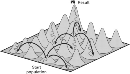
A problem which is often encountered in engineering is the determination of an optimum for a set of complex equations. the experimenter in Fig. 3.1 has defined a proving ground and now searches for the optimum, in this example represented by the highest point of the surface. there are several different approaches to solve this problem. they work on a global or a local scale and they can be deterministic or stochastic.

3.1 Experimenter searching for the optimum. (adapted from Rechenberg, 2003)
A global deterministic search will eventually in all cases be successful but may be extremely time-consuming (Fig. 3.2). A global stochastic search will lead in almost all cases to a viable solution, normally near the optimum (Fig. 3.3) and is much quicker than the former approach. A local deterministic search with a gradient process can also produce a useful solution but can also end in a local optimum far away from the global optimum (Fig. 3.4). A local stochastic search has a greater chance to succeed with a slightly higher computing time. this strategy is based on the so-called evolutionary algorithms which are the main subject of this chapter (Fig. 3.5).
3.2 Deterministic search. (adapted from Rechenberg, 2003)

3.3 Global stochastic search. (adapted from Rechenberg, 2003)
3.4 Local deterministic search. (adapted from Rechenberg, 2003)
3.5 Local stochastic search with evolutionary algorithms. (adapted from Rechenberg, 2003)
3.2 Biological background
Evolutionary algorithms follow the principles laid down by Darwin (1859) and Wallace (1871). they described the biological processes omnipresent in nature where individuals within a population compete for resources (e.g. food). Individuals better adapted to their environment than others have a higher chance of reproducing and thus passing on the genes that made them fitter to their offspring. Within a few generations, the genetic trait favouring a certain behaviour or any other evolutionary advantage spreads within the population. this also works even if several traits are required to actually produce an advantage. this process was called by Darwin 'the survival of the fittest' (Darwin, 1859).
3.2.1 Basics of genetics
the hereditary traits of a living being are encoded in genes that are copied during reproduction and passed on to the individuals of the next generation. Owing to mutation, different variants (alleles) of these genes are generated. this leads either to a slight change of a certain trait (e.g. red instead of yellow petals of a flower) or to completely new traits (e.g. resistance against vermin). this range of variations together with a recombination of the genes gradually leads to differences between the individuals within a population despite their being the offspring of the same parents. the process of a changing relative frequency of the alleles, which leads to traits becoming more common or scarce within a population, is called evolution. this change occurs due to natural selection or by accident. Natural selection is based on different survival and reproduction ratios of the individuals owing to their different traits. the so-called genetic drift is caused by random mutations of the individuals, leading to a higher percentage of a certain trait within the population.
The principles of inheritance of traits (genetics) were discovered by Mendel (1866). He assumed that 'the parental factors, combined in the zygote, do not lose their identity, but are recombined in the next generation'. The respective genetic information is binary encoded and can be recombined during reproduction. Normally, the binary encoded genes are fully passed on to the next generation. A true mixture therefore cannot occur in nature. The offspring always resembles the parents in a specific trait. For example, combining seeds of plants with red and yellow petals does not result in orange petals but again in red or yellow petals. Figure 3.6 shows this principle for three subsequent generations. Parents with diploid genes AA and aa generate offspring with genes Aa. When this offspring is recombined, the second and subsequent generations consist of individuals with diploid genes AA, Aa and aa with differing frequency. In many cases, certain traits are generated by different genes. the combination of seeds of plants with red and yellow petals can therefore nevertheless result in plants with orange petals.

Mendel's research results were not recognized by the scientific community until the early 1900s when they were rediscovered by von tschermak (1900), de Vries, (1906) and Correns, (1912). this later led to the establishment of genetics as a science. De Vries enunciated the theory of mutation stating that evolution is driven by randomly occurring variations of the genetic code of organisms. this, together with the theory of natural selection, today forms the basis of modern evolution theory.
3.2.2 Evolutionary theory
The development of the classical evolutionary theory is often attributed to Charles Darwin and his major publication ' On the origin of species by means of natural selection' (Darwin, 1859). However, there were also other scientists, e.g. Alfred R. Wallace and Jean-Baptiste de Lamarck, who made important contributions to the theory of evolution (Wallace, 1871; de Lamarck, 1909). Wallace's approach was similar to Darwin's whereas Lamarck assumed that in the course of many generations, all animals had a tendency to develop to higher levels which implies that evolution is a constantly progressing process.
As many more individuals of each species are born than can possibly survive, and as, consequently, there is a frequently recurring struggle for existence, it follows that any being, if it vary however slightly in any manner profitable to itself, under the complex and sometimes varying conditions of life, will have a better chance of surviving, and thus be naturally selected. From the strong principle of inheritance, any selected variety will tend to propagate its new and modified form.
These principles are called 'survival of the fittest' and 'natural selection'. the computer model described below which is commonly used today is based upon them.
In natural evolution, the binary encoded information is changed from generation to generation by mutation and recombination. During recombination, gene sequences consisting of bases are exchanged between adjacent DNA strands (crossing-over). this leads to a change in the order of the bases and thereby can alter traits. Recombining gene sequences by crossing-over can hence be advantageous (repair of damaged gene parts) but it can also lead to unwanted effects.
3.2.3 Chemical basics of inheritance
The discovery of the structure of deoxyribonucleic acid (DNA) as the carrier of genetic information by James Watson, Francis Crick, Maurice Wilkins and Rosalind Franklin led to a deeper understanding of the chemical principles behind inheritance (Watson and Crick, 1953). they found that genetic information is stored in the so-called bases (adenine, thymine, guanine, cytosine) that always come in pairs as shown in Fig. 3.7.

The genetic information is stored in the sequence of the bases and can therefore be read and copied very easily. If an error occurs during reading or copying, the coded information is changed. this is called a mutation. Figure 3.8 shows two common ways to create a mutation: exchanging a base for another (top) and deleting a base thus changing also the order of all subsequent base triplets (bottom). this can cause havoc in a gene as all information behind the deleted base is completely altered.

3.2.4 Genotype and phenotype
Friedrich L. A. Weismann, a German evolutionary biologist, introduced two new terms into evolutionary science: genotype and phenotype (Weismann, 1885). the genotype comprises the genetic makeup of an individual responsible for its traits. the phenotype represents the observable characteristics of an individual, also called morphology. Changing the genotype leads to a different phenotype which in turn may lead to an individual which is better adapted to its environment. this increases its changes to successfully reproduce which in turn leads to a propagation of this genotype. The benefit of a genotypic mutation of a single individual or a group of individuals does not become apparent before the interaction with the environment.
In contrast to Lamarck's theory that phenotypes change themselves through aiming to achieve an optimum (e.g. lengthening of a giraffe's neck to reach leaves higher up), changes in nature normally occur without purpose. By natural selection, non-purposeful alterations of genotypes can lead to phenotypes that are better adapted to a changed environment, thus indirectly optimizing the phenotype. An alteration of the genotype can of course also lead to non-viable solutions (individuals). If they survive, they decrease the quality of the genetic pool in the short run. But these individuals can turn out to be much better adapted to a changing environment than their relatives which previously had a competitive edge thus giving the whole population a better chance of survival. Figure 3.9 illustrates that: a small population (small genetic variation between individuals) can lead to a dead end if the environment changes (top); a larger population (greater genetic variation between individuals) may survive even a dramatic change of the environmental conditions because it contains viable solutions that were previously not relevant (bottom).

A typical example from nature is the peppered moth Biston betularia. Its light-coloured kind was perfectly adapted to birch trees, while its melanic kind was easy prey to birds. With the beginning of industrialization and huge amounts of coal being burned, birch trees in England turned black, which gave the black kind suddenly the competitive edge. So, evolution in nature is neither purely accidental (genotypic changes) nor purely goal-oriented (phenotype alteration). Only the combination of both principles leads to evolutionary progress.
3.3 Mathematical models of evolution strategy
At first sight, it seems to be a contradiction to use the term 'strategy' in the context of 'evolution'. As has been pointed out, the power of natural evolution lies in the fact that by accidental, non-strategic changes of parameters (genes), a system (population of individuals) can be constantly improved. However, the term 'evolution strategy' is commonly used in the scientific world of optimization problems and therefore also used here. When designing a mathematical model to emulate nature, there normally is a strategy behind it, so the term is justified in this context. Applying these principles, adaptive, self-optimizing systems can be designed to determine a solution for a given system of equations.
When imitating biological evolution in a computer-based model, it is not the main goal to truly copy the processes occurring in nature. The main focus is on applying the same principles that are the basis of natural evolution or at least to come close. Depending on the problem to be solved, the model resembles more or less nature's example. Each individual in a mathematical model represents a possible solution to a given problem. The parameters to-be-optimized are normally pooled in a vector consisting of binary or real numbers. Depending on how accurately it solves the problem, the vector is assigned a so-called fitness score. This is equivalent to real organisms in nature competing for resources where some are better adapted thus having a higher chance of getting them, e.g. food.
The first mathematical models of this kind were developed in the 1960s and 1970s. Owing to the limited computer performance in these days and other difficulties, there are only a few examples of successful applications, which were not used on a broad scale until recently. this is obvious when looking at the number of publications in that field over the last 20 years (Fig. 3.10).

In general, two different approaches can be distinguished: John H. Holland of University of Michigan, Ann Arbor, USA, developed the so-called genetic algorithms (GA) that describe the heredity transmission in nature in a mathematical model using binary vectors (Holland, 1992). Ingo Rechenberg and Hans-Paul Schwefel of technical University Berlin, Germany, invented the so-called evolution strategy which is based on the same principles of 'survival of the fittest' and 'natural selection' (Rechenberg, 1974, 1994; Schwefel, 1995). they do not use binary encoding but real numbers to describe the individuals, hence leaving the path of nature but simplifying the approach as a whole, especially for engineers.
3.3.1 Basics
Before applying the principles of natural evolution using a mathematical model, certain terms need to be introduced:
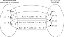
• Environment E: E stands for the environment with its boundary conditions in which the system in question is located, or, biologically spoken, in which the individuals live.
• Individuals k: A limited number of genotypes whose phenotypical interpretation p(k) interacts with the environment.
• Structure-altering operators o: they represent a limited number of operators by which the genotypes of the individuals can be altered.
• Fitness score and benchmark function B: the degree of adaptation of an individual to its environment or to certain boundary conditions can mathematically be described by a fitness score /. the better adapted an individual is, the higher its fitness score. For each phenotype p, the benchmark function B calculates its fitness score / according to / = B(π). The assessment of the fitness is based on the response R of the environment E on the phenotype p of the individual.
• Adaptation algorithm A: This algorithm modifies the genotype k of an individual through operators o as a reaction to the success of the phenotype p in the environment.
Starting with the genotype k(t) of the individual at point t, the phenotype p(k(t)) is derived. the interaction of the phenotype p with the environment E results in a reaction R(t) of the environment. In the next step, based on this reaction, the fitness value / of the phenotype is calculated applying the benchmark function B(π). After the selection of the fittest individuals according to /, the adaptation algorithm A changes the genotype k(t) and creates a new individual k(t + 1) = o(k(t)).
Figure 3.11 shows three subsequent steps of this mathematical model. It is important to note that the increment of the evolutionary changes in each step need not necessarily be constant. Moreover, the step size can be influenced on purpose by adjusting the operators o. Out of the genetic pool G(t) at point t, the adaptation algorithm A creates a new (modified) genetic pool G(t + 1). This in turn leads to a new population of individuals p(t + 1) where the population p(t + 1) is better adapted to the environment (or at least not worse) than the population p(t). This adaptation process does not stop until a previously set termination criterion T(p) is achieved. This is the case when a certain number of evolutionary cycles is completed or at least one individual has a fitness score f which reaches a pre-set value. This leads to the scheme of the evolutionary algorithm, as shown in Fig. 3.12. For the initialization of the genotypes, either a random combination of numbers or an already viable solution can be used to create the first generation of the individuals (vectors).

3.3.2 Evolution strategies
The principles as described above form the basis for all successfully applied evolution algorithms or strategies. In order to clearly characterize the different strategies, Rechenberg and others devised a commonly used notation which is described in this section (Rechenberg, 1974) and illustrated in Fig. 3.13.
(1 + 1) evolution strategy
This is the simplest version of an evolution strategy. In the first step, a single individual is created and a copy of it is reproduced. Both are vectors consisting of real numbers (see above). In the next step, the copied individual is slightly changed (mutation) by adding small positive or negative values to the vector's components if it is encoded in real numbers. If it is binary encoded, a small number of 0 are replaced by 1 and vice versa. Both individuals are assessed using the benchmark function B. The better an individual meets the set criteria for a viable solution, the higher its fitness value f. The principle of survival of the fittest determines which individual is promoted to the next round (selection), where an exact copy of it is produced again so that the next evolutionary cycle can start. If both individuals, original and copy, have the same fitness value f, one is chosen at random and the other one is eliminated from the gene pool.
These steps are repeated until an acceptable solution is found. This is a commonly used approach if it is unclear whether the best individual at the end of the evolutionary cycles, the best solution, is a global or only a local optimum. Then, in most cases, it is absolutely acceptable if the solution is sufficiently near the optimum where 'sufficiently near' is a matter of perspective. Other common abortion criteria are the completion of a preset number of cycles (generations) or the maximum computing time for the simulation as a whole. This kind of evolution strategy does not have a population of individuals in the true sense but gradually changes the genotype of a single individual by mutation.
(μ + λ) evolution strategy
This approach is a generalization version of the (1 + 1) evolution strategy where not only a single individual but a whole population is created. λ denotes the number of parental individuals, λ stands for the number of children created in each cycle or generation, with λ≥ π≥ 1. The single steps are similar in principle to the (1 + 1) evolution strategy. In the first step, λ individuals from the parent individuals are selected with equal probability and hence λchildren individuals are created which are copies of their respective parents. A repeated selection of the same parent individual is possible and even necessary in the case of λ> π. In the second step, the λ children are altered by mutation and assessed together with all parent individuals. The best μ individuals are then selected as parents for the next generation.
This strategy ensures that the quality of the best individual of the population after each cycle cannot decrease since the best individual always survives even if it has not been selected to create a child individual (Fig. 3.13). Therefore, the (μ + λ) strategy often ends in a local optimum with most individuals close to it.

3.13 Evolution strategies according to Rechenberg (1974) and Schwefel (1995).
(μ, λ) evolution strategy
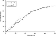
The (μ, λ) strategy overcomes this problem. After λ individuals have been selected for reproduction in the first step, all parent individuals are deleted. Then, the λ children are assessed according to their fitness value λ and μ individuals are selected as parents for the subsequent generation. This approach is closer to nature as there are no immortal individuals thus making it easier for the algorithm to leave a good, but still local, optimum. The progress of the simulation over time can be assessed using a benchmark function which calculates the fitness value λ of the best individual after each cycle (generation).
Figure 3.14 shows a typical example for the (μ + λ) and the (μ, λ) strategies over time. It is apparent that the quality of the best individual oscillates for the (μ, λ) strategy since parent individuals that have a better fitness compared to their children are nevertheless deleted. In contrast, with the (μ + λ) strategy, the fitness f of the best individual of each generation can never decrease. In the end, the final result is very similar for both approaches, with the (μ, λ) strategy probably leading to a more stable result as it normally avoids local optima. The size of the oscillation of the quality function depends on the mutation increment. If this value is small, normally the deviation of the quality function is also small.
in many cases, an evolution strategy is carried out using several independent populations of individuals. After each step, only the 'best' population survives whereas the others are deleted. Each surviving population creates daughter populations which are then subjected to mutation and benchmarked after the next cycle where only the best population survives and so forth, as shown in Fig. 3.15. Both the (μ + λ) and the (μ, λ) strategies can be combined to the (μ # λ) strategy if the selection process is not important. the symbol # then denotes either '+' or ‘;’
3.15 Evolution strategy with independent populations. (adapted from Rechenberg, 2003)
(μ/p#λ) evolution strategy
in contrast to the approaches as described above, this strategy applies the concept of sexual reproduction. the principle is very similar to those above, the main difference being that children are not produced by copying single parent individuals but by combining the genotypes of p parent individuals with p > 1 (Fig. 3.13). thus, a whole group of parents takes part in the reproduction process of a single child. the parents are selected either at random (roulette wheel) or depending on their fitness value / where fitter parents have a greater chance to reproduce than the others (see next page).
3.3.3 Recombination
Since each genotype vector consists of numbers, there is a wide range of possibilities to generate children out of the selected p parent individuals. A commonly used approach is the roulette wheel where the size of the section that each parent individual occupies is directly related to its relative fitness value. Hence, the chance of fitter individuals to be selected as parents when the ball rolls is higher than for less adapted individuals. Nevertheless, even badly suited individuals have a chance to reproduce and to pass on their genes, which in the end may be crucial to find the optimal solution. This especially applies to multi-scale problems where not only one single gene but many genes determine the overall fitness of a solution. As shown in Fig. 3.16, we have:
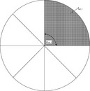
with f(Pi) = fitness value of phenotype of individual i.
Also, an element of chance can be introduced by selecting some of the parent individuals at random from the whole population while disregarding their respective itness values. This can increase the convergence speed of the whole population, when, for example, only one or two individuals of a population of 30 are generated this way.
In Fig. 3.17a, the single genes of both parents are combined completely thus generating a child consisting of genes of both parents. In this example, the genes (in order from the top) 1, 4 and 7 are taken from parent individual 1 whereas the others come from parent individual 2. In Fig. 3.17b, the genes of the child consist in equal parts of the parental genes according to:

with i = position of gene in vector.
Figure 3.17c shows the creation of child genes with different percentages for each parent:
If the percentage of each parental gene passed on to the child differs from gene to gene, then we have

and pi = recombination factors, according to Fig. 3.17d.
The recombination factors pi themselves are normally calculated by taking into account the fitness scores f1 and f2 of the parent individuals according
An alternative is to set the recombination factors at random though this often increases the number of generations needed to reach the optimum but may reduce the number of mutations required (see below). In any case, this approach where information of single genes (numbers) is actually mixed leaves the path of nature. Nevertheless, in many cases it works better than the classic approach where genes are only exchanged.
3.3.4 Mutation
Mutation plays an important part in evolutionary processes. Without mutation, in a mathematical model, children could never be created outside the space spanned by the parent individuals. When adding a small percentage of mutation to a child, this is possible. The mutation of single genes in nature is a process that normally takes place in small steps. In other words, children usually resemble their parents. Large, erratic alterations are very rare. Thus, in a mathematical model of evolution, the so-called mutation increment is kept to small values. Often, normally or uniformly distributed values are used.
Figure 3.18 depicts a reproduction process similar to that as shown in Fig. 3.17d, with the addition of a mutation component. Hence

The parameter ϑ is called mutation increment. Its value is normally in the range of ϑ = [0; 0.2], but greater values are not uncommon. Especially at the beginning of the reproduction process, this can lead to quick progress towards the global optimum. Theoretical considerations by Rechenberg (2003) and Schwefel (1995) show that on average, about one-fifth of all mutations should lead to an improvement of the population fitness. If this value is exceeded, the mutation increment should be increased; if it is below that value, the mutation increment needs to be decreased.
In self-regulating mutative increment control, the mutation increment needs to be adjusted depending on the specific problem at hand. Since this is very time-consuming, a better approach is to automatically optimize it by applying evolution strategy. Hence, the mutation increment becomes itself part of either each vector of the individuals or of the population vector as a whole and is thus optimized together with the population consisting of all individuals.
3.3.5 Selection pressure and population waves
These are two crucial factors influencing the outcome of the evolution process. Selection pressure is defined as
This allows the value S to be varied by adjusting μ and λ between the extreme values 0 (highest pressure) and 1 (lowest pressure). If the number of children λ exceeds the number of parents μ, then there is a surplus of children and hence the selection pressure is high. If the number of children equals the number of parents, then, for example in the (μ + λ) strategy, all children survive and the selection pressure is nil.
With population waves, a changing number of individuals can be simulated. This is achieved by either systematically or randomly changing the number μ of surviving individuals after each cycle which become the parents of the next generation. If the selection pressure is to be kept constant, λ must be adjusted to keep S constant.
In the context of population size and lifespan, depending on the problem to be solved, normally a number of 10 to 50 individuals is fully sufficient to find a viable solution within a couple of hundred generations. If it is unclear what the solution looks like, it can be sensible to start with a larger number of individuals in order to quickly reach the area of the optimum solution. When that is reached, which can be seen by the slowing down of the progress of the benchmark function, the number of individuals is reduced. The lifespan of individuals can be set to just one generation or be limited to a certain value in the range of 2 to 10 generations. Hence, very fit individuals are kept for a certain time to include them into the reproduction process thus generating fit children. On the other hand, this can lead to a complete standstill of the process as a local optimum may attract the majority of individuals. This local optimum is then very difficult to leave. This behaviour is also called unwanted genetic drift.
3.3.6 Summary
In general, according to Rechenberg (1994), Schwefel (1995) and the author's own experience, the number of children λ should exceed the number of parents by a factor of between 5 and 10. Selection pressure should be set to values in the range of 0.2 to 0.3. For easy-to-solve problems, the (1 # 5) evolution strategy normally works well. For more difficult problems, the (1 # 10) evolution strategy together with a self-regulative mutative increment control is more advisable (see Section 3.3.4). Figure 3.19 summarizes the evolution strategy and shows the different steps as described earlier that are carried out subsequently.

3.19 Steps during evolution (recombination, mutation, selection). (adapted from Rechenberg, 2003)
3.4 Genetic algorithms
John H. Holland developed the so-called genetic algorithms (GA) parallel to Rechenberg's evolution strategy. There, the individuals are not encoded with vectors consisting of real numbers but binary as sequences of 0 and 1. The individuals are often called chromosomes. They are created from parents using the crossing-over method where whole sequences of 0 and 1 are exchanged to produce new vectors. Mutations are also possible, when 0 is converted to 1 and vice versa (Fig. 3.20). The selection process follows the same principles as described earlier.
A fundamental difference is the selection of the parent individuals following the principle of 'survival of the fittest'. This means that parents with a good fitness value automatically have a better statistical chance to be selected for reproduction than those with bad fitness values. This aspect can also be taken into account in the evolution strategy. A self-regulating mutative increment control is difficult to implement, which is also different from Rechenberg's approach.
There are a large number of publications describing applications in engineering and textiles in particular that use GAs and only a very few that apply Rechenberg's evolution strategy (see Section 3.6). The reason for this may be due to the fact that Holland's method was easier to implement in a computer program at the time it was developed and thus spread quicker than Rechenberg's approach. With today's computing power however, the higher complexity of the latter method no longer poses an obstacle. This, together with its great advantages, which lie especially in a much better and easier fit of a 'real numbers problem', should give Rechenberg's method a competitive edge in many applications.
3.5 Comparison of evolutionary algorithms and iteration processes
There is a range of aspects in which classical iteration processes and evolutionary algorithms compete. Since the optimum solution is normally not known, usually all equations of the system at hand are set to zero for all these methods. All solutions found can then be compared with the nil-vector and hence easily be benchmarked.
3.5.1 Speed
Iteration processes, the most common being the so-called hill-climbing method, are very slow compared with evolutionary algorithms. This is due to the fact that in iterations, the solution is improved within a large number of normally very small steps. This implies that a large number of solutions needs to be calculated until a viable solution is found. Even if the distance between the current solution and the desired solution is large, the steps are often still small and all solutions in the vicinity of the current solution are also calculated.
Here, evolutionary algorithms have a competitive edge: if the current solution greatly differs from the prospective solution, then solutions near the current individual are no longer considered and solution areas a certain distance away from the current position are investigated. This behaviour can be controlled by setting the recombination and the mutation factors to certain values. Then, only those regions are further analysed, in which the difference between an individual and the optimum solution is below a given value. This often leads to either the global optimum or a local optimum which is often a sufficiently good solution.
3.5.2 Accuracy
Applying evolutionary algorithms always leads to a viable solution if carried out properly and if such a solution exists at all. But this solution is almost never the global optimum for most engineering problems.
3.5.3 Reproducibility
A variation of the starting individuals (vectors) of the evolutionary algorithm normally leads to different results. Even if the starting individuals were the same, since mutation changes the genes at random, the final results normally differ. With iteration processes, this problem is smaller. On the other hand, this phenomenon can be used to calculate different solutions to the problem which then serve as the starting points of another evolutionary cycle. In most cases, the deviation between the solutions is very small which shows that reproducibility normally is within acceptable limits.
3.5.4 Boundary conditions
In order to increase the processing speed of an iterative calculation or to even start the calculation, often boundary conditions are required. This in turn leads to a limitation of the parameters investigated and of the area in which the solution is searched, hence possible solutions are excluded. When using evolutionary algorithms, there are no boundary conditions needed as the number of parameters that can be optimized simultaneously is much larger. In addition, the solution area is not limited so the chance of excluding a good solution from the start is nil. This is a major advantage of evolutionary algorithms.
3.5.5 Summary
In summary, the main advantages of evolutionary algorithms over iteration processes are:
3.6 Applications of evolutionary algorithms to textile technology
In recent years, evolutionary algorithms have been used successfully to solve technical problems for a wide range of applications. That includes the optimization of design of aircrafts (Hansen and Horst, 2008), the bows of cargo ships (Rechenberg, 2003), antennae (Kim et al., 2011), formula 1 racing cars (Anon., 2004) and many more. In textile technology, there have also been several successful applications that are briefly described in this chapter. Most approaches employ Holland's method of binary encoding. This is surprising as Rechenberg's principles in these cases would be much easier to use and to program than to Holland's model, according to the author's experience.
3.6.1 Texturing process
Texturing is a process to give crimp to flat filament yarns in order to improve their elasticity and handle. The yarn is twisted, heated and cooled to set the twist (Fig. 3.21). In the predominantly used false-twist texturing process, the yarn is damaged during twist insertion caused by friction between yarn and texturing discs in the false twister. Several attempts have been made to create a mathematical model of the actual twist insertion. The respective equation systems were solved using iterative methods (Olbrich, 1993). Major emphasis was put on the optimization of the design of the discs (size, shape, number) to minimize friction and hence the yarn damage thereby increasing production speed (Veit et al., 1998). A significant drawback of applying these iterative methods was the necessity to take boundary conditions into account, which in turn limits the possible solutions as described previously. Therefore, an evolutionary algorithm was applied.
Genotype and phenotype
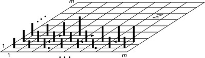
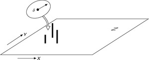
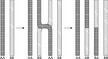
Experiments show that the yarn takes the shortest route through the false twister. Hence, the yarn is divided into small sections and the coordinates (x, y, z) of the middle of these sections are regarded as the genotype vector. The length of the yarn path through the false twister is then taken as the phenotype. The shorter the path of an individual the better its fitness and thus the greater are its chances of passing on its genotypical information to the next generation. The genotypes are varied by changing the coordinates of the vector. The only boundary condition to be taken into account is that the yarn cannot be inside the discs. It is hence allowed for the yarn to either touch the discs or to hover slightly above them. This is not possible with iterative methods and opens up a whole new range of possible solutions. Figure 3.22 shows a disc within the false twister together with a typical yarn path which is divided into single points.

Number of individuals and lifespan
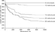
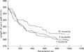
In this example, the lifespan of individuals was not limited in order not to lose a good solution. The evolution process itself was stopped after 5000 cycles (generations) as the improvement of the best solution in each step was then only marginal. Figure 3.23 shows the results of the yarn path length after 1000 generations for a different number of individuals. It is apparent that in this case 30 individuals are sufficient.
Recombination factor
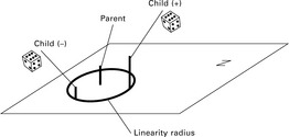
Children were generated using the principles as described above with a variable percentage of the genes of each parents (see Fig. 3.17d). In Fig. 3.24, the yarn length of the best individual after 5000 generations is depicted together with the number of parents that were used to generate children. It is obvious that using only two parents results in the best children. A larger number of parent individuals leads to worse solutions, as non-optimal genes are also taken into account, thus downgrading the result in this example. A pure mutation is apparently also a sensible approach leading to the second best result in this example.

Size of the gene pool
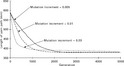
Another important factor is the size of the gene pool from which the parents are taken to create a child. Figure 3.25 shows the yarn length of the best individual after 5000 generations depending on the size of the gene pool. When the two parents are selected out of the best six individuals of the previous generation following the principles as described previously, the result is considerably worse in comparison when only the two best parental individuals of the gene pool are selected to create a child. This is due to the fact that the variety of the parental genes is large. Hence, here the genes of 'unfit' individuals have a negative effect on the children's fitness.

Mutation increment
In order to further improve the fitness of the children, a mutation component was added to the children. The value of the mutation increment (ratio) has great influence on the course of the evolution process but not so much on the final result (see Fig. 3.26). A large mutation increment quickly leads to a good result. After 5000 generations, this plus has disappeared when comparing the final result with those achieved with a smaller mutation step. Therefore, in the beginning of the evolution process, a large mutation increment can be advantageous but should then be gradually decreased when the area where the optimum is located is reached in order to avoid missing a good solution by accident.
Number of mutants
Children can be created using the principles of recombination (see Fig. 3.17a-d) or by simply mutating a single parent individual. The number of these pure mutants relative to the number of children also determines the outcome of the evolution process as is shown in Fig. 3.27. Here, 15 children were created in each generation with the number of pure mutants varying between 1 and 10. It is apparent that a too large percentage of mutants leads to unsatisfying results whereas a small number (1 to 3) leads to equally good solutions.
Importance of mutants for the evolutionary progress
Mutants are often crucial for the progress of the evolutionary process as is shown in Fig. 3.28. Here, the length of the yarn path of the best individual of each generation if shown for 2500 generations. An upright black line indicates that the best individual of each generation is a mutant, a white line indicates that it is a child created by pure recombination. It is apparent that with rare exceptions, the best individual of each generation is a mutant. This does not imply, though, that children created by recombination have a low fitness value. In contrast, a thorough analysis shows that the mutants which are the best individual of each generation are mostly themselves descendants of parents that were created applying pure recombination. Hence both, mutants and recombined children, are crucial to ensure evolutionary progress.

Final algorithm and settings
Based on the findings as described above, the evolutionary process was divided into several stages as shown in Table 3.1. The last column shows the resolution of the yarn path. This stands for the number of sections into which the yarn path is divided. The coordinates of the respective middle of each section (x, y, z) are used to create the genotype of each individual yarn path.

Reproducibility of the results
The element of chance plays an important role in evolution as was previously discussed. Hence, the final result of an evolution process always differs even if the starting point was the same for two cycles. The differences are normally very small after a certain amount of generations and can therefore normally be neglected.
Robustness
Since no boundary conditions are needed when applying an evolutionary algorithm, the starting point for the calculation is irrelevant for the final result. this is illustrated in Fig. 3.29. the course of the expected yarn path is reversed and taken as the starting point. Even starting from this extremely bad solution, the algorithm is able to come up with a viable result within 5000 generations.
3.6.2 Weaving machine
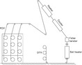
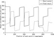
An evolutionary algorithm was employed to optimize the machine settings during weaving by Wolters and Gries (2001). the principle of this approach was called 'AUTOWARP' and is shown in Fig. 3.30. Fabric data are fed into a simulation program and the expected warp tension (1) is calculated based on data from weaving mills by using a neural network. It is not possible to directly relate the course of the warp tension during weft insertion with a specific machine setting. Therefore, another simulation program is used that is able to calculate the warp tension based on the machine settings. As is shown in Fig. 3.31, that calculated warp tension (2) is compared with the desired warp tension (1). If the difference is sufficiently small, the optimum machine setting has been found. If this is not the case, those machine settings that led to the closest correlation with the warp tension (1) are then used as parents for the next generation of machine settings. the resulting warp tension (2) is again calculated, compared with warp tension (1) and so forth until both warp tensions coincide sufficiently well. Then, the optimized machine setting to produce the desired fabric has been found. this system was successfully tested in weaving mills and is now a commercially available product. It shows the great potential of GA to help finding optimum machine settings even for highly complicated processes and machines. It is one of the rare examples of an application in textiles of Rechenberg's method.
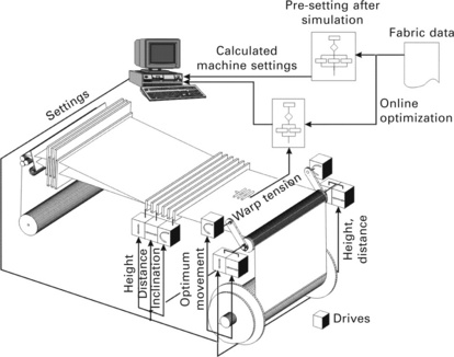
3.30 Design of AUTOWARP to optimize weaving machine settings. (adapted from Wolters and Gries, 2001)

3.31 Evolutionary algorithm to determine optimized machine settings (adapted from Wolters, 2002)
3.6.3 Degumming of kenaf
Zheng and Du (2009) combined GAs with a neural network in order to reduce the chemical residues on kenaf fibres, thus decreasing environmental pollution. In a first step, they trained a neural network to find feasible and acceptable machine settings. Then, they defined an objective function fGA given by
This they used in a second step to further optimize the machine settings. A verification of the results by experiments showed that machine set-up was indeed improved compared to the original state.
3.6.4 Staple fibre spinning
Liu and Yu (2008) also combined GAs according to Holland with a backpropagation neural network but with a different approach from the one outlined in Zheng and Du (2009). They created a so-called genetic neural network where the weight and threshold matrices were optimized using GAs. One major aim was to optimize the evenness of wool rovings (output) depending on wool top oil content, wool top moisture, fibre mean diameter and ten other parameters (input). A chromosome was defined which included the weight and threshold values of all nodes. This led to a chromosome string length of 106 as a network was used with 13 input, 7 hidden and 1 output neurons. Based on the performance of each respective neural network, gradually optimized settings for weight and threshold matrix were found. As Fig. 3.32 shows, the genetically optimized neural network led to slightly better results than a conventional network. This approach is most interesting and certainly worthy of pursuing further for a wide range of applications where the classic method to optimize the weight factors of an ANN is too time consuming.
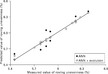
3.32 Comparison between roving evenness predicted with neural network (filled symbols) and with genetic neural network (open symbols). (adapted from Liu and Yu, 2008)
3.6.5 Carpet pattern design
Zamani et al. (2009) used GAs to generate new carpet patterns in a very innovative way. According to the authors, traditional methods to generate hand-made carpet patterns include artistic imitation and combination of traditional patterns, the adaptation of painting tables and the general generation of patterns through a creative process. This is time-consuming and expensive. An interesting alternative is the use of GAs. In a first step, each pattern is encoded in a chromosome consisting of information about corner, brink and medallion (centre of the carpet) motives, the respective sizes and colours. In total, 28 genes are encoded using a binary function as shown in Fig. 3.33.

3.33 Chromosome encoding of a pattern. (adapted from Zamani et al., 2009)
In order to create a new population, different crossover and mutation operations are employed leading to new chromosomes and thus to new patterns. These patterns are then presented to the user for assessment, thus attributing a fitness value to the patterns. Depending on this value, the respective individuals of the pattern population are more likely to be selected for reproduction of the next pattern generation. The best pattern is always kept. This process leads quickly to new and innovative patterns as shown in Fig. 3.34 (initial population) and Fig. 3.25 (patterns after four generations). In order not to lose high-rated patterns, certain parts of a pattern can be set manually to a defined value by the user and thus taken out of the evolution process.

To further improve this method, a neural network is used. It is trained with the characteristics of a pattern as input and the grading of the user as output. Hence, it is possible to actually predict the expected fitness value of a certain pattern thus avoiding unwanted patterns and directing the process towards higher graded motives.
3.6.6 Improving the structure of an ANN
in a similar approach as described above, Admuthe et al. (2009) used a GA to optimize the settings of an ANN which was used to link fibre properties and resulting yarn characteristics. in contrast to the method described in Section 3.6.1, they binary encoded the structural and other parameters in a chromosome as depicted in Fig. 3.36 using Holland's principle. Learning rate, momentum factor, number of generations and other parameters were assigned numbers selected from predefined values in order to limit the number of possible combinations. Then, the classic method of GA was employed as described earlier. the number of individuals was set to 100 with each representing seven parameters of the ANN setting. After only 50 generations, the achieved result with regard to mean error of the ANN for all patterns was below the set absolute threshold of 0.01 (Fig. 3.37). this method is a very useful approach for users of ANNs who lack extensive experience about adjusting the crucial factors for a successful training of an ANN properly and hence are not able to define optimal settings of an ANN directly.
3.36 Encoding ANN structure and other parameters in a chromosome. (adapted from Admuthe et al., 2009)

3.37 Optimizing the training of an ANN with evolution strategy. (adapted from Admuthe et al., 2009)

3.6.7 Spinning of staple fibre yarns
In another paper, Admuthe and Apte (2009) applied a genetic algorithm based on Holland's approach to further improve the results of a neural network. The basic idea is shown in Fig. 3.38. In a first step, they trained a backpropagation network with fibre properties and the resulting yarn characteristics as is common practice. They then employed a genetic algorithm to match as best as possible the predicted fibre properties with those fibres that are actually on stock. The fitness function of the GA was described by
3.38 ANN-GA-LP model. (adapted from Admuthe and Apte, 2009)
where f(x) is the fitness value, Ri represents the predicted property, Ai the property of available fibres and n stands for the number of parameters describing the fibre. The fibre properties themselves were encoded according to Fig. 3.39.
![]()
3.39 Binary encoding of fibre properties in a chromosome. (adapted from Admuthe and Apte, 2009)
A linear programming (LP) method was applied to further improve the quality of the predictions by calculating an optimized blend consisting of a wide range of different fibres. This was used to reduce the cost by replacing expensive fibres with cheap fibres while still keeping the required properties of the blend. This is a novel approach that led to a distinctive improvement of the predictions with regard to costs and could, according to the authors, be especially useful for mills with a wide range of yarns from different cotton varieties.
3.6.8 Other applications
Recent papers include the optimization of the design of apparel production lines (Wang and Chen, 2010), a system that automatically separates colour printed fabrics (Kuo et al., 2009), the detection of the layout of colour yarns from the colour pattern of yarn-dyed fabrics (Pan et al., 2010) and a system that helps to detect the courses of breakdowns during the weaving process (Lin, 2009). The range of possible applications of GA in textiles is huge, since in many textile-related problems, there are often many parameters interacting and relations that cannot be described with mathematical equations. Most researchers use Holland's approach which is, as mentioned above, strange as Rechenberg's method appears to be easier to use but is apparently unknown to many scientists.
3.7 Practical advice in applying evolutionary methods
The settings of the evolutionary algorithm, e.g. number of individuals in the population, crossing-over factor and mutation factor, are not crucial in terms of whether an optimal solution will be found or not. The basic mechanism of evolution strategy was found to be very robust (Grefenstette, 1986) and a variation of these parameters normally only marginally affects the overall performance. Depending on the problem, either binary or real number encoding of the individuals can be advantageous. In general, one would expect real number encoding better suited to solve problems involving complex equations. If a binary problem needs to be solved, then Holland's approach may be easier to implement.
Much more critical is to find a suitable fitness function. In the ideal case, the fitness function is smooth and regular with only one optimum. In reality, this is, unfortunately, hardly ever the case. Otherwise one could just as well employ a hill-climbing algorithm. Hence, it is normally very difficult to find the global optimum when there are a large number of local optima. In order to cut short a normally very time-consuming process, the 'resolution' of the search space can be changed as was shown in Section 3.6.1. In the following steps, the resolution can be refined until it reaches the actual values. Another possibility is to define intermediate goals that will eventually lead to the overall target. This can be done by giving fitness points to solutions that reach some of the overall targets to the degree with which they fulfil them or by just counting the number of sub-targets that they achieve.
A common problem is premature convergence of the algorithm. This can be solved by introducing a sufficiently high number of mutants with a suitable mutation increment as was described earlier. This also works for slowly converging populations when all individuals of a population are located around the optimum and the gradient of the fitness scores is insufficient to actually push some individuals towards the global target.
In general, it is always advisable to run the evolution strategy more than once in order to get an idea whether the found solutions are similar or located in totally different regions of the search space which does happen at times. In the latter case, repeated runs of the algorithm will eventually lead to the global or at least an acceptable optimum. Different methods are described in detail in Beasley et al. (1993a, 1993b) which also give an excellent introduction into GA in general.
3.8 Web references for software tools
There is a wide range of software tools and general information on the world wide web. The following links are a selection of useful websites.
Free GA software
http://www.oocities.org/geneticoptimization/
http://download.cnet.com/Genetic-Algorithm-Library/3000-2070_4-10822277.html
http://www.brothersoft.com/genetic-algorithm-and-direct-search-tool-226443.html (Matlab© extension)
http://genetic-algorithm-labview.fyxm.net/ (Labview© extension)
Other sources
http://dces.essex.ac.uk/staff/rpoli/gp-field-guide/ ('Field Guide to Genetic Programming')
http://www.obitko.com/tutorials/genetic-algorithms/ (comprehensive tutorial)
http://samizdat.mines.edu/ga_tutorial/ga_tutorial.ps (online tutorial)
3.9 References
Admuthe, L.S., Apte, S.D., Optimization of spinning process using hybrid approach involving ANN, GA and linear programming. Proceedings of the 2nd Bangalore Annual Compute Conference, COMPUTE'09. 2009.
Admuthe, L., Apte, S.D., Admuthe, S., Topology and parameter optimization of ANN using genetic algorithm for application of textiles. Proceedings of the 5th IEEE International Workshop on Intelligent Data Acquisition and Advanced Computing Systems: Technology and Applications, IDAACS, 2009:278–282. [2009].
Anon. Mit Darwin zum Formel-1-Sieg. Der Spiegel. 2004; 26:132.
Beasley, D., Bull, D.R., Martin, R.R. An overview of genetic algorithms. Part 1: fundamentals', University of Wales, College of Cardiff, University Computing, 1993. 1993; 15(2):58–69.
Beasley, D., Bull, D.R., Martin, R.R. An overview of genetic algorithms. Part 2: Research topics', University of Wales, College of Cardiff, University Computing, 1993. 1993; 15(4):170–181.
Correns, K.Die Bestimmung und Vererbung des Geschlechtes nach Neuen Versuchen mit Höheren Pflanzen. BiblioBazaar, 1912. [(new edition, 2009)].
Darwin, C.On the Origin of Species by Means of Natural Selection, or the Preservation of Favoured Races in the Struggle for Life. London: Murray, 1859. [New edition by Sterling Publishing (2008)].
de Lamarck, J.B. Philosophie Zoologique. Paris: Verdiere; 1909.
De Vries, H., Species and Varieties, Their Origin by MutationLectures Delivered at the University of California by Hugo de Vries. Nabu Press, 1906. [(new edition, 2010)].
Grefenstette, J.J. Optimization of control parameters for genetic algorithms. IEEE Trans SMC. 1986; 16:122–128.
Hansen, L., Horst, P. Multilevel optimization in aircraft structural design evaluation. Computers and Structures. 2008; 86(1–2):104–118.
Holland, J.H. Adaptation in Natural and Artificial Systems, 2nd edition. MIT Press; 1992.
Kim, K.-T., Kwon, S.-H., Ko, J.-H., Kim, H.-S. An optimal design of a 19.05GHz high gain 44 array antenna using the evolution strategy. Transactions of the Korean Institute of Electrical Engineers. 2011; 60(4):811–816.
Kuo, C.-F.J., Kao, C.-Y., Chiu, C.-H. Integrating a genetic algorithm and a self-organizing map network for an automatically separating color printed fabric system. Textile Research Journal. 2009; 79(13):1235–1244.
Lin, J.-J. A genetic algorithm-based solution search to fuzzy logical inference for breakdown causes in fabric inspection. Textile Research Journal. 2009; 79(5):394–409.
Liu, G., Yu, W.-D. Integrated genetic neural network and its application in the worsted fore-spinning process. Proceedings of the 4th International Conference on Natural Computation. 2008; vol. 5:554–558.
Mendel, G., Versuche über Pflanzenhybriden Bd. IV,. Verhandlungen des naturforschenden Vereines in Brünn. Abhandlungen, 1866:3–47. [English translation: Druery, C.T and William Bateson (1901). 'Experiments in plant hybridization'. Journal of the Royal Horticultural Society, 26, 1–32.].
Olbrich, A. Chemiefasern-Textilindustrie. 1993; 43/95(issue 10):828–830.
Pan, R., Gao, W., Liu, J., Wang, H. Genetic algorithm-based detection of the layout of color yarns. Journal of the Textile Institute. 2010; 102(2):172–179.
Rechenberg, I. Evolutionsstrategie. Frommann-Holboog; 1974.
Rechenberg, I. Evolutionsstrategie 94. Frommann-Holboog; 1994.
Rechenberg, I. Evolutionsstrategie, script to lecture. TU Berlin; 2003.
Schwefel, H.-P. Evolution and Optimum Seeking (Sixth-Generation Computer Technology). Wiley VCH; 1995.
Veit, D., Laourine, E., Wulfhorst, B. New disc-geometry in the false-twist texturing process to reduce the snow production. Chemical Fibers International. 1998; 48:89–90.
Von Tschermak, E.Versuche über Pflanzenhybriden. Nabu Press, 1900. [(new edition, 2010).].
Wallace, A.R. Contributions to the Theory of Natural Selection. Macmillan and Company; 1871.
Wang, B., Chen, S., The optimized design of apparel streamline based on genetic algorithm. Proceedings of the 6th International Conference on Natural Computation, 2010.
Watson, J.D., Crick, F. Molecular structure of nucleic acids: a structure for deoxyribose nucleic acid. Nature. 1953; 171:737–738.
Weismann, F.A.On Germinal Selection as a Source of Definite Variation. BiblioBazaar, 1885. [(new edition, 2008).].
Wolters, T. Verbesserte Webmaschineneinstellungen mittels Simulationsrechnungen. Germany: RWTH Aachen University; 2002. [Dissertation].
Wolters, T., Gries, T. Intelligent adjustment device for looms. Proceedings of the International Textile Congress. 2001; 1:310–317.
Zamani, F., Amani-Tehran, M., Latifi, M. Interactive genetic algorithm-aided generation of carpet pattern. Journal of the Textile Institute. 2009; 100(6):556–564.
Zheng, L., Du, B. Neural network modeling for bio-enzymatic degumming on kenaf. 5th International Conference on Natural Computation, ICNC 2009. 2009; vol. 2:223–226.