The simplest neural network we could imagine is composed of a single linear function, and is known as a perceptron (Rosenblatt, Frank. The perceptron, a perceiving and recognizing automaton Project Para. Cornell Aeronautical Laboratory, 1957):

Here, w is a set of weights for each of the input features in the column vector x, and b is the intercept. You may recognize this as being very similar to the formula for the SVM we examined in Chapter 5, Putting Data in its Place – Classification Methods and Analysis, when the kernel function used is linear. Both the function above and the SVM separates data into two classes depending upon whether a point is above or below the hyperplane given by w. If we wanted to determine the optimal parameters for this perceptron using a dataset, we could perform the following steps:

While this model is easy to understand, it has practical limitations for many problems. For one, if our data cannot be separated by a hyperplane (they are not linearly separable), then we will never be able to correctly classify all data points. Additionally, all the weights are updated with the same rule, meaning we need to learn a common pattern of feature importance across all data points. Additionally, since the outputs are only 1 or 0, the Perceptron is only suitable for binary classification problems. However, despite these limitations, this model illustrates some of the common features of more complex neural network models. The training algorithm given above adjusts the model weights based on the error of classification tuned by a learning rate, a pattern we will see in more complex models as well. We will frequently see a thresholded (binary) function such as the preceding one, though we will also relax this restriction and investigate the use of other functions.

How can we develop this simple Perceptron into a more powerful model? As a first step, we can start by combining inputs from many individual models of this kind.

Just as a biological brain is composed of individual neuronal cells, a neural network model consists of a collection of functions such as the Perceptron discussed previously. We will refer to these individual functions within the network as neurons or units. By combining the inputs from several functions, blended using a set of weights, we can start to fit more complex patterns. We can also capture nonlinear patterns by using other functions than the linear decision boundary of the Perceptron. One popular choice is the logistic transform we previously saw in Chapter 5, Putting Data in its Place – Classification Methods and Analysis. Recall that the logistic transform is given by:

Here, w is a set of weights on the elements of the vector x, and b is an offset or bias, just as in the Perceptron. This bias serves the same role as in the Perceptron model, increasing or decreasing the score calculated by the model by a fixed amount, while the weights are comparable to regression coefficients we have seen in models from Chapter 4, Connecting the Dots with Models – Regression Methods. For simpler notation in the following derivation, we can represent the value wx+b as a single variable z. As in the logistic regression model from Chapter 5, Putting Data in its Place – Classification Methods and Analysis, this function maps the input x into the range [0,1] and can be visually represented (Figure 1) as an input vector x (consisting of three green units) connected by lines (representing the weights W) to a single blue unit (the function F(z)).

In addition to increasing the flexibility with which we can separate data through this nonlinear transformation, let us also adjust our definition of the target. In the Perceptron model, we had a single output value 0 or 1. We could also think of representing this as a two-unit vector (shown in red in Figure 1), in which one element is set to 1 and the other 0, representing which of the two categories a data point belongs to. This may seem like an unnecessary complication, but it will become very useful as we build increasingly complex models.

With these modifications, our model now consists of the elements show in Figure 1. The logistic function takes input from the three features of x represented by the vector at the top of the diagram, combines them using the logistic function with the weights for each element of x given by W1, and returns an output. This output is then used by two additional logistic functions downstream, represented by the red units at the bottom of the diagram. The one on the left uses the output of the first function to give a score for the probability of class 1. On the right, a second function uses this output to give the probability of class 0. Again, the input from the blue unit to the red units is weighted by a vector W2. By tuning the value of W2 we can increase or decrease the likelihood of activting one of the red nodes and setting its value to 1. By taking the maximum over these two values, we get a binary classification.

Figure 1: Architecture of a basic single-layer neural network

This model is still relatively simple, but has several features that will also be present in more complex scenarios. For one, we now actually have multiple layers, since the input data effectively forms the top layer of this network (green nodes). Likewise, the two output functions form another layer (red nodes). Because it lies between the input data and the output response, the middle layer is also referred to as the hidden layer of the network. In contrast, the bottom-most level is called the visible layer, and the top the output layer.

Right now, this is not a very interesting model: while it can perform a nonlinear mapping from the input x using the logistic function, we only have a single set of weights to tune from the input, meaning we can effectively only extract one set of patterns or features from the input data by reweighting it. In a sense, it is very similar to the Perceptron, just with a different decision function. However, with only a few modifications, we can easily start to create more complex mappings that can accommodate interactions between the input features. For example, we could add two more neurons to this network in the hidden layer, as shown in the Figure 2. With these new units, we now have three potentially different sets of weights for the elements of the input (each representing different weighting of the inputs), each of which could form a different signal when integrated in the hidden layer. As a simple example, consider if the vector represented an image: the hidden neurons on the right and left could receive weights of (1,0,0) and (0,0,1), picking up the edges of the image, while the middle neuron could receive weight (0,1,0) and thus only consider the middle pixel. The output probabilities of the two classes in the output layer now receive contributions from all three hidden neurons. As a result, we could now adjust the weight parameters in the vector W2 to pool contributions from the three hidden units to decide the probability of the two classes

Figure 2: A more complex architecture with three units in the hidden layer

Even with these modifications, the Figure 2 represents a relatively simple model. To add more flexibility to the model we could add many more units to the hidden layer. We could also extend this approach to a problem with more than two classes by adding more units to the output layer at the bottom of the diagram. Also, we have only considered linear and logistic transformations thus far, but as we will see later in this, chapter there are a wide variety of functions we could choose.

However, before we consider more complex variations on this design, let us examine the methodology to determine the proper parameters for this model. The insertion of the intermediate layers means we can no longer rely on the simple learning training algorithm that we used for the Perceptron model. For example, while we still want to adjust the weights between the input and hidden layer to optimize the error between the prediction and the target, the final prediction is now not given by the output of the hidden layer, but the output layer below it. Thus, our training procedure needs to incorporate errors from the output layer in tuning hidden levels of the network.

Given the three layer network shown in Figure 2, how can we determine the best set of weights (W) and offsets (b) that map our input data to the output? As with the Perceptron algorithm, we can initially set all our weights to random numbers (a common strategy is to sample them from a normal distribution with mean of 0 and standard deviation of 1). We then follow the flow of the arrows in the network from top to bottom, computing the logistic transform for each node at each stage until we arrive at the probabilities of each of the two classes.

To adjust our randomly chosen parameters to better fit the output, we can calculate what direction the weights should move to reduce the error between the predicted and observed response y, just as with the Perceptron learning rule. In Figure 2 we can see two sets of weights we need to adjust: those between the input and hidden layer (W1) and those between the hidden layer and the output (W2).

Let us start with the simpler case. If we are tuning the bottom-most weights (between the output and the hidden layer), then we want to find the change in the errors (the difference between the prediction and the real value of the output) as we alter the weights. For now, we will use a squared error function to illustrate:

Here, yi is the actual value of the label, and F(zi) represents one of the red neurons in the output layer (in this example, a logistic function). We want to calculate the change in this error function when we adjust the weight (one of the lines connecting the hidden blue and output red neurons in the Figure 2), represented by the variable Wij, where i and j are indices for the red and blue neurons connected by a given weight. Recall that this weight is actually an argument of the variable z (since z=wx+b), representing the input to the function logistic F. Because the variable w is nested inside the logistic function, we cannot calculate the partial derivative the error function with respect to this weight directly to determine the weight update Δw.

To see this, recall an example from calculus if we wanted to find the derivative of the function with respect to x:

We would need to first take the derivative with respect to ez, then multiply by the derivative of z with respect to x, where z=x2, giving a final value of . This pattern, given more generally by:

This is known as the chain rule, since we chain together derivatives in calculations with nested functions. In fact, though are example was for only a single level of nesting, we could extend this to an arbitrary number, and would just need to insert more multiplication terms in the formula above.

Thus, to calculate the change in the error function E when we change a given weight wij, we need to take the derivative of the error function with respect to F(z) first, followed by the derivative of F(z) with respect to z, and finally the derivative of z with respect to the weight wij. When we multiply these three partial derivatives together and cancel terms in the numerator and denominator, we obtain the derivative of the error function with respect to the weight. This, the partial derivative of this error with respect to a particular weight w between one the outputs i and one of the hidden neurons j is given using the chain rule described previously:

Now that we have the formula to determine the derivative of the error function with respect to the weight, let us determine the value of each of these three terms. The derivative for the first term is simply the difference between the prediction and the actual response variable:

For the second term, we find that the partial derivative of the logistic function has a convenient form as a product of the function and 1 minus the function:

Finally for the last term we have simply,

Here, F(z)j is the output of the hidden layer neuron j. To adjust the weight wij, we want to move in the opposite direction to which the error is increasing, just as in the stochastic gradient descent algorithm we described in Chapter 5, Putting Data in its Place – Classification Methods and Analysis. Thus, we update the value of the weight using the following equation:

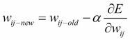
Where α is a learning rate. For the first set of weights (between the input and the hidden layer), the calculation is slightly more complicated. We start again with a similar formula as previously:

Where wjk is the weight between a hidden neuron j and a visible neuron k. Instead of the output, F(z)i, the partial derivative of the error with respect to the weight is now calculated with respect to the hidden neuron's output F(z)j. Because the hidden neuron is connected to several output neurons, in the first term we cannot simply use the derivative of the error with respect to the output of the neuron, since F(z)j receives error inputs from all these connections: there is no direct relationship between F(z)j and the error, only through the F(z)i of the output layer. Thus, for hidden to visible layer weights we need to calculate the first term of this partial derivative by summing the results of applying the chain rule for the connection from each output neuron i:

In other words, we sum the partial derivatives along all the arrows connecting wjk to the output layer. For the hidden to visible weights, this means two arrows (from each output to the hidden neuron j).

Since the input to the hidden neuron is now the data itself in the visible layer, the third term in the equation becomes:

This is simply an element of the data vector x. Plugging in these values for the first and third terms, and using the gradient descent update given previously, we now have all the ingredients we need to optimize the weights in this network. To train the network, we repeat the following steps:

This process is known as back-propagation (Bryson, Arthur E., Walter F. Denham, and Stewart E. Dreyfus. Optimal programming problems with inequality constraints. AIAA journal 1.11 (1963): 2544-2550; Rumelhart, David E., Geoffrey E. Hinton, and Ronald J. Williams. Learning representations by back-propagating errors. Cognitive modeling 5.3 (1988): 1; Bryson, Arthur Earl. Applied optimal control: optimization, estimation and control. CRC Press, 1975; Alpaydin, Ethem. Introduction to machine learning. MIT press, 2014.) because visually the errors in prediction flow backward through the network to the connection weights w from the input. In form, it is quite similar to the Perceptron learning rule that we discussed at the beginning of this chapter, but accommodates the complexity of relating the prediction error to the weights between the hidden and visible layers, which depend on all output neurons in the example we have illustrated.

In the examples described previously and illustrated in Figures 1 and 2, the arrows always point exclusively forward from the input data to the output target. This is known as a feed-forward network, since the movement of information is always in one direction (Hinton, Geoffrey, et al. Deep neural networks for acoustic modeling in speech recognition: The shared views of four research groups. IEEE Signal Processing Magazine 29.6 (2012): 82-97). However, this is not a hard requirement—if we had a model in which arrows moved both forward and backward in the visible layer (Figure 3), we could in a sense have a generative model not unlike the LDA algorithm discussed in Chapter 6, Words and Pixels – Working with Unstructured Data:

Figure 3: A Restricted Boltzman Machine (RBM) as the top two levels of the neural network from Figure 2

Instead of simply generating a predicted target in the output layer (a discriminative model), such a model could be used to draw samples from the presumed distribution of the input data. In other words, just as we could generate documents using the probability model described in LDA, we could draw samples from the visible layer using the weights from the hidden to the visible layer as inputs to the visible neurons. This kind of neural network model is also known as a belief network, since it can be used to simulate the 'knowledge' represented by the network (in the form of the input data) as well as perform classification. A visible and hidden layer in which there is a connection between each neuron in both layers is a kind of model known more generally as a Restricted Boltzman Machine (RBM) (Smolensky, Paul. Information processing in dynamical systems: Foundations of harmony theory. No. CU-CS-321-86. COLORADO UNIV AT BOULDER DEPT OF COMPUTER SCIENCE, 1986; Hinton, Geoffrey E., James L. Mcclelland, and David E. Rumelhart. Distributed representations, Parallel distributed processing: explorations in the microstructure of cognition, vol. 1: foundations. (1986).).

In addition to providing a way for us to understand the distribution of the data by simulating samples from the space of possible input data points that the network has been exposed to, RBMs can form useful building blocks in the deep networks that we will construct using additional hidden layers. However, we are presented with a number of challenges in adding these additional layers.

Even the architecture shown in Figures 2 and 3 is not the most complex neural network we could imagine. The extra hidden layer means we can add an additional interaction between the input features, but for very complex data types (such as images or documents), we could easily imagine cases where capturing all interactions of interests might require more than one layer of blending and recombination to resolve. For example, one could imagine a document dataset where individual word features captured by the network are merged into sentence fragments features, which are further merged into sentence, paragraph, and chapter patterns, giving potentially 5+ levels of interaction. Each of these interactions would require another layer of hidden neurons, with the number of connections (and weights which need to be tuned) consequently rising. Similarly, an image might be resolved into grids of different resolution that are merged into smaller and larger objects nested within each other. To accommodate these further levels of interaction by adding additional hidden layers into our network (Figure 4), we would end up creating an increasingly deep network. We could also add additional RBM layers like we described . Would this increased complexity help us learn a more accurate model? Would we still be able to compute the optimal parameters for such a system using the back-propagation algorithm?

Figure 4: Multilayer neural network architecture

Let us consider what happens in back-propagation when we add an extra layer. Recall that when we derived the expression for the change in the error rate as a function of the weights in the first layer (between visible and the first hidden layer), we ended up with an equation that was a product of the weights between the output and hidden layer, as well as the weights in the first layer:

Let us consider what happens when the first term (the sum over the errors from the output layer) is <1. Since this formula is a product, the value of the entire expression also decreases, meaning we will change the value of wjk by very small steps. Now recall that to calculate the change in the error with respect to a visible to hidden connection wjk we needed to sum over all the connections from the output to this weight. In our example, we had just two connections, but in deeper networks we would end up with extra terms such as the first to capture the error contribution from all the layers between the hidden and output. When we multiply by more terms with value < 1, the value of the total expressions will increasingly shrink towards 0, meaning the value of the weight will get updated hardly at all during the gradient step. Conversely, if all these terms have value > 1, they will quickly inflate the value of the whole expression, causing the value of the weight to change wildly between gradient update steps.

Thus, the change in error as a function of the hidden to visible weights tends to approach 0 or increase in an unstable fashion, causing the weight to either change very slowly or oscillate wildly in magnitude. It will therefore take a longer time to train the network, and it will be harder to find stable values for weights closer to the visible layer. As we add more layers, this problem becomes worse as we keep adding more error terms that make it harder for the weights to converge to a stable value, as increasing the number of terms in the product representing the gradient has a greater likelihood of shrinking or exploding the value.

Because of this behavior adding more layers and using back-propagation to train a deep network are not sufficient for effectively generating more complex features by incorporating multiple hidden layers in the network. In fact, this problem also known as vanishing gradients due to the fact that the gradients have a greater chance of shrinking to zero and disappearing as we add layers, was one of the major reasons why multilayer neural network remained practically infeasible for many years (Schmidhuber, Jürgen. Deep learning in neural networks: An overview. Neural Networks 61 (2015): 85-117.). In a sense, the problem is that the outer layers of the network 'absorb' the information from the error function faster than the deeper layers, making the rate of learning (represented by the weight updates) extremely uneven.

Even if we were to assume that we are not limited by time in our back-propagation procedure and could run the algorithm until the weights finally converge (even if this amount of time were impractical for real-world use), multilayer neural networks present other difficulties such as explaining away.

The explaining away effect concerns the tendency for one input unit to overwhelm the effect of another. A classic example (Hinton, Geoffrey E., Simon Osindero, and Yee-Whye Teh. A fast learning algorithm for deep belief nets. Neural computation 18.7 (2006): 1527-1554) is if our response variable is a house jumping off the ground. This could be explained by two potential inputs piece of evidence, whether a truck has hit the house and whether an earthquake has occurred nearby (Figure 5):

Figure 5: Explaining away causes imbalanced weighting in deep networks

If an earthquake has occurred, then the evidence for this being the cause of the house's movement is so strong that the truck collision evidence is minimized. Simply put, knowing that an earthquake has occurred means we no longer need any additional evidence to explain the house moving, and thus the value of the truck evidence becomes negligible. If we are optimizing for how we should weight these two sources of evidence (analogous to how we might weight the inputs from hidden neurons to an output unit), the weight on the truck collision evidence could be set to 0, as the earthquake evidence explains away the other variable. We could turn on both inputs, but the probability of these two co-occurring is low enough that our learning procedure would not optimally do so. In effect, this means that the value of the weights are correlated with whether the hidden neurons (represented by each evidence type) are turned on (set to 1). Thus, it is difficult to find a set of parameters that does not saturate one weight at the expense of the other. Given the problem of vanishing gradients and explaining away, how could we hope to find the optimal parameters in a deep neural network composed of many layers?

Both the vanishing gradient and explaining away effects are in a sense are caused by the fact that it is difficult to find an optimal set of weights for large networks if we start from a set of random values and perform back-propagation. Unlike the logistic regression objective function we saw in Chapter 5, Putting Data in its Place – Classification Methods and Analysis, the optimal error in a deep learning network is not necessarily convex. Thus, following gradient descent through back-propagation for many rounds is not guaranteed to converge to globally optimal value. Indeed, we can imagine the space of the Error function as a multidimensional landscape, where the elevation represents the value of the error function and the coordinates represent different values of the weight parameters. Back-propagation navigates through different parameter values by moving up or down the slopes of this landscape, which are represented by the steps taken with each weight update. If this landscape consisted of a single steep peak located at the optimal value of the weights, back-propagation might quickly converge to this value. More often, though, this multidimensional space could have many ravines and valleys (where the error functions dips and rises in irregular ways with particular set of weights), such that it is difficult for a first-order method such as back-propagation to navigate out of local minima/maxima. For example, the first derivative of the error function could change slowly over a valley in the error function landscape, as the error only gradually increases or decreases as we move in or around the valley. Starting in a random location in this landscape through the standard random initialization of the weight variables might leave us in a place where we are unlikely to ever navigate to the optimal parameter values. Thus, one possibility would be to initialize the weights in the network to a more favorable configuration before running back-propagation, giving us a better chance of actually finding the optimal weight values.

Indeed, this is the essence of the solution proposed by research published in 2006 (Hinton, Geoffrey E., Simon Osindero, and Yee-Whye Teh. A fast learning algorithm for deep belief nets. Neural computation 18.7 (2006): 1527-1554). Instead of fitting a multi-layer neural network directly to the response variable for a dataset (in this case, the digits represented by a set of images of hand-drawn numbers) after random initialization of the weight variables, this study suggested that the network weights could be initialized through a pre-training phase that would move them closer to the correct values before running back-propagation. The networks used in this study contained several RBM layers, and the proposed solution was to optimize one RBM at a time through the following steps, which are illustrated in Figure 6:

This pre-training procedure has the practical effect that the network is initialized with weights that are in the general shape of the input data. The fact that this procedure is employed on a single layer at a time avoids some of the vanishing gradient problems discussed previously, since only a single set of weights is considered in each step. The problem of explaining away is also minimized due to the matching of weights as described in step 5. Going back to our example of house movement, the relative strength of the earthquake and truck weights would be represented in the first layer of the deep belief network. In the next phase of pre-training, these weights would be inverted through the matrix transpose, undoing the explaining away effect in the higher layer. This pattern is repeated in sequential layers, systematically removing the correlation between the value of the weights and the likelihood of the connected hidden unit being activated.

Once this pretraining is complete, a back-propagation-like approach is used as described for simpler networks, but the weights now converge much quicker to stable values because they have started at a more optimal, instead of random, value.

Even using the pretraining approach described previously, it can be computationally expensive to optimize a large number of parameters in deep networks. We also potentially suffer from the same problem as regression models with large numbers of coefficients, where the large number of parameters leads the network to overfit the training data and not generalize well to data it has not previously seen.

While in the case of regression, we used approaches such as Ridge, Lasso, and Elastic Net to regularize our models, for deep networks we can use an approach known as Dropout to reduce overfitting (Srivastava, Nitish, et al. Dropout: a simple way to prevent neural networks from overfitting. Journal of Machine Learning Research 15.1 (2014): 1929-1958.). The idea is relatively is simple: at each stage of tuning the weights, we randomly remove some neuron units along with their connections from the network and only update the remaining weights. As we repeat this process, we effectively average over many possible network structures. This is because with a 50% probability of dropping any given neuron at each stage from the network, each stage of our training effectively samples from 2n possible network structures. Thus, the model is regularized because we are only fitting a subsample of parameters at each stage, and similar to the random forest we examined in Chapter 5, Putting Data in its Place – Classification Methods and Analysis, we average over a larger number of randomly constructed networks. Even though dropout can reduce over fitting, it could potentially make the training process longer, since we need to average over more networks to obtain an accurate prediction.

Even though the pre-training procedure provides a way to initialize network weights, as we add layers the overall model complexity increases. For larger input data (for example, large images), this can lead to increasing numbers of weights along with each additional layer, and thus the training period may take longer. Thus, for some applications, we might accelerate the training process by intelligently simplifying the structure of our network by (1) not making a connection between every single neuron in every layer and (2) changing the functions used for neurons.

These kinds of modifications are common in a type of deep network also known as a Convotional Network (LeCun, Yann, et al. Gradient-based learning applied to document recognition. Proceedings of the IEEE 86.11 (1998): 2278-2324; Krizhevsky, Alex, Ilya Sutskever, and Geoffrey E. Hinton. Imagenet classification with deep convolutional neural networks. Advances in neural information processing systems. 2012). The name convolution comes from image analysis, where a convolution operator such as the opening and dilation operations we used in Chapter 6, Words and Pixels – Working with Unstructured Data are applied to overlapping areas of an image. Indeed, convolutional Networks are commonly applied to tasks involving image recognition. While the number of potential configurations is large, a potential structure of a convolutional network might be the following (see Figure 7):

This architecture exploits the structure of the data (examining local patterns in images), and training is faster because we only make selective connections between neurons in each layer, leading to fewer weights to optimize. A second reason that this structure can train more rapidly is due to the activation functions used in the rectification and pooling layers. A common choice of pooling function is simply the maximum of all inputs, also known as a Rectified Linear Unit (ReLU) (Nair, Vinod, and Geoffrey E. Hinton. Rectified linear units improve restricted boltzmann machines. Proceedings of the 27th International Conference on Machine Learning (ICML-10). 2010). which is:

Here, z is the input to a given neuron. Unlike the logistic function described previously, the ReLU is not bounded by the range [0,1], meaning that the values to neurons following it in the network can change more rapidly than is possible with logistic functions. Furthermore, the gradient of the ReLU is given by:

This means that gradients do not tend to vanish (unless the neuron inputs drop very low such that it is always off) or explode, as the maximum change is 1. In the former case, to prevent the ReLU from turning permanently off, the function could be modified to be leaky:

Here, α is a small value such a 0.01, preventing the neuron from ever being set to 0.

Figure 7: Convolutional neural network architecture. For clarity, connections in convolutional layer are represented to highlighted region rather than all wxhxd neurons, and only a subset of the network converging to a pooling layer neuron is shown.

Tip

Aside: Alternative Activation Functions

In addition to the linear, sigmoid, and ReLU functions discussed previously, other activation functions are also used in building deep networks. One is the hyperbolic tangent function, also known as the tanh function, given by:

The output of this function is in the range [–1,1], unlike the sigmoid or ReLU, which are in the range [0,1], and some evidence suggests that this could accelerate training of networks by allowing the average output of neurons to be zero and thus reduce bias (LeCun, Yann, Ido Kanter, and Sara A. Solla. "Second order properties of error surfaces: Learning time and generalization." Advances in neural information processing systems 3 (1991): 918-924.). Similarly, we could imagine using a Gaussian function such as the kernels we saw in Chapters 3, Finding Patterns in the Noise – Clustering and Unsupervised Learning, and Chapter 5, Putting Data in its Place – Classification Methods and Analysis, in the context of spectral clustering and SVMs, respectively. The softmax function used for multinomial regression in Chapter 5, Putting Data in its Place – Classification Methods and Analysis, is also a candidate; the number of potential functions increases the flexibility of deep models, allowing us to tune specific behavior according to the problem at hand.

While most of our discussion in this chapter involves the use of deep learning for classification tasks, these models can also be used for dimensionality reduction in a way comparable to the matrix factorization methods we discussed in Chapter 6, Words and Pixels – Working with Unstructured Data. In such an application, also known as an auto-encoder network (Hinton, Geoffrey E., and Ruslan R. Salakhutdinov. Reducing the dimensionality of data with neural networks. Science 313.5786 (2006): 504-507), the objective is not to fit a response (such as binary label), but to reconstruct the data itself. Thus, the visible and output layers are always the same size (Figure 8), while the hidden layers are typically smaller and thus form a lower-dimensional representation of the data that can be used to reconstruct the input. Thus, like PCA or NMF, autoencoders discover a compact version of the input that can approximate the original (with some error). If the hidden layer was not smaller than the visible and output, the network might well just optimize the hidden layer to be identical to the input; this would allow the network to perfectly reconstruct the input, but at the expense of any feature extraction or dimensionality reduction.

Figure 8: Autoencoder network architecture

In the examples we have discussed above, the learning rate for the parameters at each stage is always a fixed value α. Intuitively, it makes sense that for some parameters we may want to adjust the value more aggressively, while others less. Many optimizations have been proposed for this sort of tuning. For example, Adative Gradient (AdaGrad) (Duchi, John, Elad Hazan, and Yoram Singer. Adaptive subgradient methods for online learning and stochastic optimization. Journal of Machine Learning Research 12.Jul (2011): 2121-2159.) uses a learning rate for each parameter based on the past history of gradients for a given parameter:

Where Gt represents the sum of squares of all gradients of a particular parameter, gt is the gradient at the current step, and ε is a smoothing parameter. Thus, the learning rate at each stage is the global value α, multiplied by a fraction that the current gradient represents of the historic variation. If the current gradient is high compared to historical updates, then we change the parameter more. Otherwise, we should change it less. Over time, most the learning rates will shrink toward zero, accelerating convergence.

A natural extension of this idea is used in AdaDelta (Zeiler, Matthew D. ADADELTA: an adaptive learning rate method. arXiv preprint arXiv:1212.5701 (2012)), where instead of using the full history of gradient updates G, we, at each step, replace this value with the average of the current gradient and the historical average gradient:

The expression for Adagrad then uses the above formula in the denominator instead of Gt. Like Adagrad, this will tend to reduce the learning rate for parameters that are not changing significantly relative to their history.

The TensorFlow library we will examine in the following also provides the Adaptive Moment Estimation (ADAM) method for adjusting the learning rate (Kingma, Diederik, and Jimmy Ba. Adam: A method for stochastic optimization. arXiv preprint arXiv:1412.6980 (2014).). In this method, like AdaDelta, we keep an average of the squared gradient, but also of the gradient itself. The update rule is then as follows:

Here, the weighted averages as in AdaDelta, normalized by dividing by a decay parameter (1-β). Many other algorithms have been proposed, but the sample of methods we have described should give you an idea of how the learning rate may be adaptively tuned to accelerate training of deep networks.

Figure 9: Recurrent Neural Network (RNN) and Long Short Term Memory (LSTM) architectures.

Now that we have seen how a deep learning network is constructed, trained, and tuned through a variety of optimizations, let's look at a practical example of image recognition.