
In our previous example of logistic regression, we assumed implicitly that every point in the training set might be useful in defining the boundary between the two classes we are trying to separate. In practice we may only need a small number of data points to define this boundary, with additional information simply adding noise to the classification. This concept, that classification might be improved by using only a small number of critical data points, is the key features of the support vector machine (SVM) model.
In its basic form, the SVM is similar to the linear models we have seen before, using the following equation:
where b is an intercept, and β is the vector of coefficients such as we have seen in regression models. We can see a simple rule that a point X is classified as class 1 if F(x) ≥ 1, and class -1 if F(x) ≤ –1. Geometrically, we can understand this as the distance from the plane to the point x, where β is a vector sitting orthogonal (at a right angle) to the plane. If the two classes are ideally separated, then the width between the two classes represented by 1/![]() is as large as possible; thus, in finding the optimal value of β, we would to minimize the norm
is as large as possible; thus, in finding the optimal value of β, we would to minimize the norm ![]() . At the same time, we want to minimize the error in assigning labels to the data. Thus, we can have a loss function that minimizes the tradeoff between these two objectives:
. At the same time, we want to minimize the error in assigning labels to the data. Thus, we can have a loss function that minimizes the tradeoff between these two objectives:

where y is the correct label of x. When x is correctly classified, y(xβ+b) ≥ 1, and we overall subtract from the values of L. Conversely, when we incorrectly predict x.
Note that the || here represent the Euclidean norm, or:
y(xβ+b) < 1, and we thus add to the value of L. If we want to minimize the value of L, we could find the optimal value of β and b by taking the derivative of this function and setting it to 0. Starting with β:

Similarly, for b:

Plugging these back into the loss function equation we get:

Two things are important here. First, only some of the α need to be nonzero. The rest can be set to 0, meaning only a small number of points influence the choice of optimal model parameters. These points are the support vectors that give the algorithm its name, which lie along the boundary between the two classes. Note that in practice we would not use the above version of the error function, but rather a soft-margin formulation in which we use the
hinge loss:
This means that we only penalize points if they are on the wrong side of the separating hyperplane, and then by the magnitude of their misclassification error. This allows the SVM to be applied even in cases where the data is not linearly separable by allowing the algorithm to make mistakes according to the hinge loss penalty. For full details please consult references (Cortes, Corinna, and Vladimir Vapnik. Support-vector networks. Machine learning 20.3 (1995): 273-297; Burges, Christopher JC. A tutorial on support vector machines for pattern recognition. Data mining and knowledge discovery 2.2 (1998): 121-167.).
Second, we now see that the solution depends on the inputs x only through the product of individual points. In fact, we could replace this product with any function K(xi,xj), where K is a so-called
kernel function representing the similarity between xi and xj. This can be particularly useful when trying to capture nonlinear relationships between data points. For example, consider data points along a parabola in two-dimensional space, where x2 (the vertical axis) is the square of x1 (the horizontal). Normally, we could not draw a straight line to separate points above and below the parabola. However, if we first mapped the points using the function x1, sqrt(x2), we can now linearly separate them. We saw the effectiveness of this nonlinear mapping in Chapter 3, Finding Patterns in the Noise – Clustering and Unsupervised Learning, when we use the Gaussian Kernel to separate the nonlinear boundary between concentric circles using Spectral K-Means clustering.
Besides creating a linear decision boundary between data points that are not linearly separable in the input space, Kernel functions also allow us to calculate similarities between objects that have no vector representation, such as graphs (nodes and edges) or collections of words. The objects do not need to be the same length, either, as long as we can compute a similarity. These facts are due to a result known as Mercer's Theorem, which guarantees that Kernel functions which are >=0 for all pairs of inputs represent a valid inner product ![]() between inputs x mapped into a linearly separable space using the mapping represented by φ (Hofmann, Thomas, Bernhard Schölkopf, and Alexander J. Smola. Kernel methods in machine learning. The annals of statistics (2008): 1171-1220). This mapping could be explicit, such as the square root function applied to the parabolic input in the example above. However, we do not actually need the mapping at all, since the kernel is guaranteed to represent the similarity between the mapped inputs. Indeed, the mapping could even be performed in an infinite-dimensional space that we can not explicitly represent, as is the case with the Gaussian kernel we will describe as follows.
between inputs x mapped into a linearly separable space using the mapping represented by φ (Hofmann, Thomas, Bernhard Schölkopf, and Alexander J. Smola. Kernel methods in machine learning. The annals of statistics (2008): 1171-1220). This mapping could be explicit, such as the square root function applied to the parabolic input in the example above. However, we do not actually need the mapping at all, since the kernel is guaranteed to represent the similarity between the mapped inputs. Indeed, the mapping could even be performed in an infinite-dimensional space that we can not explicitly represent, as is the case with the Gaussian kernel we will describe as follows.
Now that we have covered some of the intuition behind SVMs, let us see if it can improve the performance of our classification model by fitting an SVM to the data.
For this example, we will try the default kernel function for the SVM model in scikit-learn, which is a Gaussian kernel, which you may recognize as the same equation used in a normal distribution function. We previously used the Gaussian Kernel in the context of Spectral Clustering in Chapter 3, Finding Patterns in the Noise – Clustering and Unsupervised Learning, as a reminder, the formula is:

In essence, this function translates the difference between two data points into the range 1 (when they are equal and the exponent becomes 0) and 0 (when the difference is very large and the exponent tends toward a very large negative number). The parameter γ represents the standard deviation, or bandwith, which controls how quickly the value of the function tends towards zero as the difference between the points increases. Small values of the bandwith will make the numerator a larger negative number, thus shrinking the kernel value to 0.
As we mentioned preceding, the Gaussian kernel represented mapping the inputs x into an infinite dimensional space. We can see this if we expand the value of the kernel function using an infinite series:

Thus, the Gaussian kernel captures a similarity in an infinite dimensional features space.
We fit the SVM model to the training data using the following commands:
>>> from sklearn import svm
>>> svm_model = svm.SVC(probability=True,kernel='rbf').fit(census_features_train.toarray(),census_income_train)
>>> train_prediction = svm_model.predict_proba(census_features_train.toarray())
>>> test_prediction = svm_model.predict_proba(census_features_test.toarray())
>>> fpr_train, tpr_train, thresholds_train = metrics.roc_curve(np.array(census_income_train),
   np.array(train_prediction[:,1]), pos_label=1)
>>> fpr_test, tpr_test, thresholds_test = metrics.roc_curve(np.array(census_income_test),
   np.array(test_prediction[:,1]), pos_label=1)
>>> plt.plot(fpr_train, tpr_train)
>>> plt.plot(fpr_test, tpr_test)
>>> plt.xlabel('False Positive Rate')
>>> plt.ylabel('True Positive Rate')
However, upon plotting the ROC curve for the results, we find that we have not improved very much over the logistic regression:

It may be difficult to see, but the red line in the upper left-hand corner of the image is the performance on the training set, while the blue line is the performance on the test set. Thus, we are in a situation such as we described previously, where the model almost perfectly predicts the training data but poorly generalizes to the test set.
In some sense, we were able to make progress because we used a nonlinear function to represent similarity within our data. However, the model now fits our data too well. If we wanted to experiment more with SVM models, we could tune a number of parameters: we could change kernel function, adjust the bandwidth of the Gaussian kernel (or the particular hyper parameters of whichever kernel function we chose), or tune the amount by which we penalize errors in classification. However, for our next step of algorithm optimization, we will instead switch gears and try to incorporate nonlinearity with many weak models instead of one overfit model, a concept known as boosting.
In the previous examples, we have implicitly assumed that there is a single model that can describe all the patterns present in our data set. What if, instead, a different model were best suited for a pattern represented by a subset of data, and only by combining models representing many of these smaller patterns can we can get an accurate picture? This is the intuition behind boosting—we start with a weak individual model, determine which points it correctly classifies, and fit additional models to compensate for points missed by this first model. While each additional model is also relatively poor on its own, by successively adding these weak models that capture a certain subset of the data, we gradually arrive at an accurate prediction overall. Furthermore, because each of the models in this group is fit to only a subset of the data, we have to worry less about over-fitting. While the general idea of boosting can be applied to many models, let us look at an example using the decision trees we covered in Chapter 4, Connecting the Dots with Models – Regression Methods.
Recall that in Chapter 4, Connecting the Dots with Models – Regression Methods, we achieved greater predictive power in our regression task by averaging over a set of trees with random features. Gradient boosted decision trees (Breiman, Leo. Arcing the edge. Technical Report 486, Statistics Department, University of California at Berkeley, 1997; Friedman, Jerome H. Greedy function approximation: a gradient boosting machine. Annals of statistics (2001): 1189-1232; Friedman, Jerome H. Stochastic gradient boosting. Computational Statistics and Data Analysis 38.4 (2002): 367-378.) follow a similar strategy, but instead of choosing random features with each step, we greedily optimize at each point. The general algorithm is:
- Start with a constant value, such as the average response across the input data. This is the baseline model, F0.
- Fit a decision tree h to the training data, usually limiting it to have very shallow depth, with the target as the pseudo-residuals for each point
igiven by:
- Conceptually, the pseudo-residual for a given loss function L (such as the squared error that we studied in Chapter 4, Connecting the Dots with Models – Regression Methods or the hinge loss for the SVM described above) is the derivative of the loss function with respect to the value of the current model F at a point
yi. While a standard residual would just give the difference between the predicted and observed value, the pseudo-residual represents how rapidly the loss is changing at a given point, and thus in what direction we need to move the model parameters to better classify this point. - To step 1, add the value of the tree in step 2 multiplied by an optimal step
γand a learning rateα: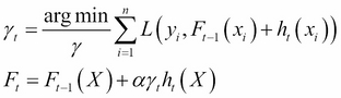
- We could either choose a
γthat is optimal for the whole tree, or for each individual leaf node, and we can determine the optimal value using a method such as the Newton optimization we discussed above. - Repeat steps 1–3 until convergence.
The goal is that by fitting several weaker trees, in aggregate they make better predictions as they sequentially are fit to compensate for the remaining residuals in the model at each step. In practice, we also choose only a subset of the training data to fit the trees at each stage, which should further reduce the possibility of over-fitting. Let us examine this theory on our dataset by fitting a model with 200 trees with a maximum depth of 5:
>>> from sklearn.ensemble import GradientBoostingClassifier
>>> gbm = GradientBoostingClassifier(n_estimators=200, learning_rate=1.0,
… max_depth=5, random_state=0).fit(census_features_train.toarray(),census_income_train)
>>> train_prediction = gbm.predict_proba(census_features_train.toarray())
>>> test_prediction = gbm.predict_proba(census_features_test.toarray())
>>> fpr_train, tpr_train, thresholds_train = metrics.roc_curve(np.array(census_income_train),
…   np.array(train_prediction[:,1]), pos_label=1)
>>>fpr_test, tpr_test, thresholds_test = metrics.roc_curve(np.array(census_income_test),
…   np.array(test_prediction[:,1]), pos_label=1)
Now, when we plot the results, we see a remarkable increase in accuracy on the test set:
>>> plt.plot(fpr_train, tpr_train)
>>> plt.plot(fpr_test, tpr_test)
>>> plt.xlabel('False Positive Rate')
>>> plt.ylabel('True Positive Rate')

Similar to the random forest model, we can examine the importance of features as determined by the loss in accuracy upon shuffling their values among data points:
>>> np.array(expanded_headers)[np.argsort(gbm.feature_importances_)]
array(['native-country Outlying-US(Guam-USVI-etc)',        'native-country Holand-Netherlands', 'native-country Laos',        'native-country Hungary', 'native-country Honduras',        'workclass Never-worked', 'native-country Nicaragua',        'education Preschool', 'marital-status Married-AF-spouse',        'native-country Portugal', 'occupation Armed-Forces',        'native-country Trinadad&Tobago', 'occupation Priv-house-serv',        'native-country Dominican-Republic', 'native-country Hong',        'native-country Greece', 'native-country El-Salvador',        'workclass Without-pay', 'native-country Columbia',        'native-country Yugoslavia', 'native-country Thailand',        'native-country Scotland', 'native-country Puerto-Rico',        'education 1st-4th', 'education 5th-6th'
Note that this is not directly comparable to the same evaluation we performed for the logistic regression model as the importance here is not determined by whether the feature predicts positively or negatively, which is implicit in the sign of the coefficients in the logistic regression.
Also note that there is a subtler problem here with interpreting the output coefficients: many of our features are actually individual categories of a common feature, such as country of origin or education level. What we are really interested in is the importance of the overall feature, not the individual levels. Thus, to quantify feature importance more accurately, we could average the importance over all columns containing categories belonging to a common feature.
If we wanted to further tune the performance of the gbm model, we could perform a search of different values for the number of trees, the depth of those trees, the learning rate (α in the formulas above), and min_samples_leaf (which determines the minimum number of data points that need to be present to split the data form a bottom-most split, or leaf, in the tree), among others. As a rule of thumb, making deeper trees will increase the risk of over-fitting, but shallower trees will requires a larger number of models to achieve good accuracy. Similarly, a lower learning rate will also control over-fitting by reducing the contribution of any single tree to the model score, but again may require a tradeoff in more models to achieve the desired level of predictive accuracy. The balance between these parameters may be guided both by the application (how accurate the model should be to contribute meaningfully to a business problem) as well as performance considerations (if the model needs to run online in a website, for example, a smaller number of trees that occupy less memory may be beneficial and worth a somewhat reduced accuracy).