One of the weaknesses of the k-means algorithm is that we need to define upfront the number of clusters we expect to find in the data. When we are not sure what an appropriate choice is, we may need to run many iterations to find a reasonable value. In contrast, the Affinity Propagation algorithm (Frey, Brendan J., and Delbert Dueck. Clustering by passing messages between data points. science 315.5814 (2007): 972-976.) finds the number of clusters automatically from a dataset. The algorithm takes a similarity matrix as input (S) (which might be the inverse Euclidean distance, for example – thus, closer points have larger values in S), and performs the following steps after initializing a matrix of responsibility and availability values with all zeroes. It calculates the responsibility for one datapoint k to be the cluster center for another datapoint i. This is represented numerically by the similarity between the two datapoints. Since all availabilities begin at zero, in the first round we simply subtract the highest similarity to any other point (k') for i. Thus, a high responsibility score occurs when point k is much more similar to i than any other point.

Where i is the point for which we are trying to find the cluster center, k is a potential cluster center to which point i might be assigned, s is their similarity, and a is the 'availability' described below. In the next step, the algorithm calculates the availability of the datapoint k as a cluster center for point i, which represents how appropriate k is as a cluster center for i by judging if it is the center for other points as well. Points which are chosen with high responsibility by many other points have high availability, as per the formula:

Where r is the responsibility given above. If i=k, then this formula is:

These steps are sometimes described as message passing, as they represent information being exchanged by the two datapoints about the relative probability of one being a cluster center for another. Looking at steps 1 and 2, you can see that as the algorithm proceeds the responsibility will drop for many of the datapoints to a negative number (as we subtract not only the highest similarity of other datapoints, but also the availability score of these points, leaving only a few positives that will determine the cluster centers. At the end of the algorithm (once the responsibilities and availabilities are no longer changing by an appreciable numerical amount), each datapoint points at another as a cluster center, meaning the number of clusters is automatically determined from the data. This method has the advantage that we don't need to know the number of clusters in advance, but does not scale as well as other methods, since in the simplest implantation we need an n-by-n similarity matrix as the input. If we fit this algorithm on our dataset from before, we see that it detects far more clusters than our elbow plot suggests, since running the following commands gives a cluster number of 309.

>>> affinity_p_clusters = sklearn.cluster.AffinityPropagation().fit_predict(X=np.array(df)[:,1:]) 
>>> len(np.unique(affinity_p_clusters))

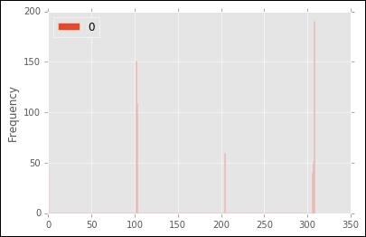
However, if we look at a histogram of the number of datapoints in each cluster, using the command:

>>> pd.DataFrame(affinity_p_clusters).plot(kind='hist',bins=np.unique(affinity_p_clusters))

We can see that only a few clusters are large, while many points are identified as belonging to their own group:

Where K-Means Fails: Clustering Concentric Circles

So far, our data has been well clustered using k-means or variants such as affinity propagation. What examples might this algorithm perform poorly on? Let's take one example by loading our second example dataset and plotting it using the commands:

>>> df = pd.read_csv("kmeans2.txt",sep="	")
>>> df.plot(x='x_coord',y='y_coord',kind='scatter')

By eye alone, you can clearly see that there are two groups: two circles nested one within the other. However, if we try to run k-means clustering on this data, we get an unsatisfactory result, as you can see from running the following commands and plotting the result:

>>> kmeans_clusters = KMeans(2).fit_predict(X=np.array(df)[:,1:])
>>> df.plot(kind='scatter', x='x_coord', y='y_coord', c=kmeans_clusters)

In this case, the algorithm was unable to identify the two natural clusters in the data—because the center ring of data is the same distance to the outer ring at many points, the randomly assigned cluster center (which is more likely to land somewhere in the outer ring) is a mathematically sound choice for the nearest cluster. This example suggests that, in some circumstances, we may need to change our strategy and use a conceptually different algorithm. Maybe our objective of squared error (inertia) is incorrect, for example. In this case, we might try k-medoids.