While we have dealt thus far with the simple of example of a two-class problem , we could imagine scenarios in which there are multiple classes: for example, predicting which of a set of items a customer will select in an online store. For these sorts of problems, we can imagine extending the logistic regression to K classes, where K > 2. Recall that taking e to the power of the logit function gives:

In a two-class problem, this value compares the ratio of the probability that Y=1 to all other values, with the only other value being 0. We could imagine running instead a series of logistic regression models for K classes, where e(Logit(x)) gives the ratio of the probability of Y = class k to any of other class. We would then up with a series of K expressions for e(Xβ) with different regression coefficients. Because we want to constrain the outcome to be in the range 0 to –1, we can divide the output of any of the K models by the sum of all K models using the formula:

This equation also known as the softmax function. It is used extensively in neural network models (which we will cover in Chapter 7, Learning from the Bottom Up – Deep Networks and Unsupervised Features). It has the nice property that even for extreme values of e(xβ) for a given class k, the overall value of the function cannot go beyond 1. Thus, we can keep outliers in the dataset while limiting their influence on the overall accuracy of the model (since otherwise they would tend to dominate the overall value of an error function, such as the squared error we used in linear regression in Chapter 4, Connecting the Dots with Models – Regression Methods).

To keep the current presentation less complex, we will examine only a 2-class problem in the following exercises. However, keep in mind that as with logistic regression, the other methods discussed in the following can be extended to work with multiple classes as well. Additionally, we will demonstrate a full multiclass problem in Chapter 7, Learning from the Bottom Up – Deep Networks and Unsupervised Features using neural networks.

Now that we have covered what logistic regression is and the problem it is designed to solve, let us prepare a dataset for use with this and other classification methods. In addition to working through a practical example of fitting and interpreting a logistic regression model, we will use this a starting point to examine other classification algorithms.

In this example, we will use a census dataset with rows representing the characteristic of an adult US citizen (Kohavi, Ron. Scaling Up the Accuracy of Naive-Bayes Classifiers: A Decision-Tree Hybrid. KDD. Vol. 96. 1996). The objective is to predict whether an individual's income is above or below the average income of $55,000 a year. Let us start by loading the dataset into a pandas data frame and examining the first few rows using the following commands:

>>> census = pd.read_csv('census.data',header=None)
>>> census.head()

Why did we use the argument (header = None) to load the data? Unlike some of the other datasets we have examined in previous chapters, the column names for the census data are contained in a separate file. These feature names will be helpful in interpreting the results, so let us parse them from the dataset description file:

>>> headers_file = open('census.headers')
>>> headers = []
>>> for line in headers_file:
>>>    if len(line.split(':'))>1: # colon indicates line is a column description
>>>        headers.append(line.split(':')[0]) # the column name precedes the colon
>>> headers = headers[15:] # the filter in the if (…) statement above is not 100 percent accurate, need to remove first 15 elements
>>> headers.append('income') # add label for the response variable in the last column
>>> census.columns = headers # set the column names in the dataframe to be extracted names

Now that we have the column names appended to the dataset, we can see that the response variable, income, needs to be re-encoded. In the input data, it is coded as a string, but since scikit-learn is unable to take a string as an input, we need to convert it into a 0 or 1 label using the following code:

>>> census.income = census.income.map( lambda x: 0 if x==' <=50K' else 1)

Here, we have used a lambda expression to apply an anonymous function (a function without a name defined in the rest of the program) to the data. The conditional expression within the map (…) call takes x as an input and returns either 0 or 1. We could just as easily have formally defined such as function, but especially for expressions we do not intend to reuse, lambda expressions provide an easy way to specify such transformations without crowding our code with a lot of functions that do not have general utility.

Let us take a moment and look at the distribution of the different income classes by plotting a histogram with income as the value on the vertical axis:

>>> census.plot(kind='hist', y='income')

Notice that observations with the label 1 are about 50 percent less prevalent than those with a label of 0. As we discussed previously, this is a situation in which a simple threshold of half in evaluating the class probabilities will lead to an inaccurate model, and we should keep this data skew in mind as we evaluate the performance later.

In addition to our outcome variable, many of the features in this dataset are also categorical: we will need to re-encode them as well before fitting our model. We can do so in two steps: first, let us find the number of unique elements in each of these columns and map them to integer values using a dictionary. To begin, we check whether each column in the data frame is categorical (dtype equal to object), and, if so, we add its index into the list of columns we want to convert:

>>> categorical_features = [e for e,t in enumerate(census.dtypes) if t=='object' ]

Now that we have the column numbers we want to convert, we need to make a mapping of each column from a string to a label from 1 to k, where k is the number of categories:

>>> categorical_dicts = []
>>> for c in categorical_features:
>>>    categorical_dicts.append(dict( (i,e) for (e,i) in enumerate(census[headers[c]].unique()) ))

Notice that we first extract the unique elements of each column and then use the enumerate function on this list of unique elements to generate the labels we need. By converting this indexed list into a dictionary where the keys are the unique elements of a column and the values are the labels, we have exactly the mapping we need to re-encode the categorical string variables in this data as integers.

Now we can create a second copy of the data using the mapping dictionary we generated above:

>>> census_categorical = census
>>> for e,c in enumerate(categorical_features):
>>>   census_categorical[headers[c]] =  census_categorical[headers[c]].
map(categorical_dicts[e].get)

Now, we can use scikit-learn's one-hot encoder to transform these integer values into a series of columns, of which only one is set to 1, representing which of the k classes this row belongs to. To use the one-hot encoder, we also need to know how many categories each of the columns has, which we can do with the following command by storing the size of each mapping dictionary:

>>> n_values = [len(d) for d in categorical_dicts] 

We then apply the one-hot encoder:

>>> from sklearn.preprocessing import OneHotEncoder
>>> census_categorical_one_hot = OneHotEncoder(categorical_features=categorical_features, n_values=n_values).fit_transform(census_categorical[headers[:-1]])

From here we have the data in the right format to fit our logistic regression. As with our examples in Chapter 4, Connecting the Dots with Models – Regression Methods, we need to split our data into training and test sets, specifying the fraction of data in the test set (0.4). We also set the random number generator seed to 0 so that we can replicate the analysis later by generating the same random set of numbers:

>>> from scipy import sparse
>>> from sklearn import cross_validation
>>> census_features_train, census_features_test, census_income_train, census_income_test = 
>>> cross_validation.train_test_split(census_categorical_one_hot, 
>>> census_categorical['income'], test_size=0.4, random_state=0)

Now that we have prepared training and test data, we can fit a logistic regression model to the dataset. How can we find the optimal parameters (coefficients) of this model? We will examine two options.

The first approach, known as stochastic gradient descent (SGD), calculates the change in the error function at a given data point and adjusts the parameters to account for this error. For an individual data point, this will result in a poor fit, but if we repeat this process over the whole training set several times, the coefficients will converge to the desired values. The term stochastic in this method's name refers to the fact that this optimization is achieved by following the gradient (first derivative) of the loss function with respect to a given data point in a random order over the dataset. Stochastic methods such as this one often scale well to large datasets because they allow us to only examine the data individually or in small batches rather than utilizing the whole dataset at once, allowing us to parallelize the learning procedure or at least not use all the memory on our machine to process large volumes of data.

In contrast, the optimization methods implemented by default for the logistic regression function in scikit-learn are known as second-order methods. SGD, because it adjusts the model parameter values using the first derivative of the error function, is known as a first-order method. Second-order methods can be beneficial in cases where the first derivative is changing very slowly, as we will see in the following, and to find the optimal value in cases where the error function follows complex patterns.

Let us look at each of these methods in more detail.

How do we find the optimal parameters for our logistic regression model using stochastic updates? Recall that we are trying to optimize the probabilities:

f we want to optimize the probability of each individual point in our dataset, we want to maximize the value of the equation, known as the Likelihood as it scores the probability of given point being class 1 (or 0) based on the model;

You can see that if the real label yi is 1, and the model gives high probability of 1, then we maximize the value of F(zi) (since the exponent of the second term is 0, making it 1, while the first term in the product is simply the value of F(zi)). Conversely, if the real label of yi is 0, then we want the model to maximize the value of (1-F(zi)), which is the probability of class 0 under the model.

Thus, each point will contribute to the likelihood by the probability of its real class. It is usually easier to work with sums than products, so we can take the logarithm of the likelihood equation and sum over all elements in the data set using:

To find the optimal value of the parameters, we just take the first partial derivative with respect to the parameters of this equation (the regression coefficients) and solve for the value of β that maximizes the likelihood equation by setting the derivative equal to 0 and finding the value of β as illustrated below:

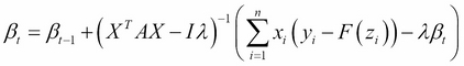
This is the direction we want to update the coefficients β in order to move it closer to the optimum. Thus, for each data point, we can make an update of the following form:

where α is the learning rate (which we use to control the magnitude by which the coefficients can change in each step – usually a smaller learning rate will prevent large changes in value and converge to a better model, but will take longer), t is the current optimization step, and t-1 is the previous step. Recall that in Chapter 4, Connecting the Dots with Models – Regression Methods we discussed the concept of regularization, in which we can use a penalty term λ to control the magnitude of our coefficients. We can do the same here: if the regularization term in our likelihood is given by (to penalize the squared sum of the coefficients, which is the L2 norm from Ridge Regression in Chapter 4, Connecting the Dots with Models – Regression Methods):

Then once we take the first derivate, we have:

And the final update equation becomes:

We can see, this regularization penalty has the effect of shrinking the amount by which we modify the coefficients β at any given step.

As we mentioned previously, stochastic updates are especially efficient for large datasets as we only have to examine each data point one at a time. One downside of this approach is that we need to run the optimization long enough to make sure the parameters converge. For example, we could monitor the change in the coefficient values as we take the derivative with respect to each data point, and stop when the values cease changing. Depending upon the dataset, this could occur quickly or take a long time. A second downside is that following the gradient of the error function along the first derivative will not always lead to the fastest solution. Second-order methods allow us to overcome some of these deficits.

In the case of logistic regression, our objective function is convex (see aside), meaning that whichever optimization method we choose should be able to converge to the global optimum. However, we could imagine other scenarios: for example, the surface of the likelihood equation plotted as a function of the inputs could vary slowly in a long ravine toward its global optimum. In such a case, we would like to find the direction to move the coefficients that is the optimal tradeoff between the rate of change and the rate of the rate of change, represented by the second derivative of the likelihood. Finding this tradeoff allows the optimization routine to traverse slowly varying regions quickly. This kind of strategy is represented by the class of so-called Newton methods, which minimizes equations of the following form:

Where f(x*) is the objective function we are trying to minimize, such as the logistic regression error, and x are the values (such as the model coefficients) that do minimize regression likelihood, x* are the inputs which optimize the value of the function (such as the optimal coefficients β), and xt are the value of these parameters at the current step of the optimization (there is admittedly some abuse of notation here: in the rest of the chapter, x are the input rows, where here we use x to represent a parameter value in a model). The name Newton method is due to the father of physics, Isaac Newton, who described an early version of this procedure (Ypma, Tjalling J. Historical development of the Newton-Raphson method. SIAM review 37.4 (1995): 531-551). The minimization involves finding the direction we should move the parameters at the current stage, xt, in order to find the minimal value of f. We can use a Taylor Expansion from Calculus to approximate the value of the preceding function:

We want to find the value of Δx which maximizes the function, since this is the direction we wish to move the parameters, just as in gradient descent. We can obtain this optimal direction by solving for the point where the gradient of the function becomes 0 with respect to Δx, to give:

Thus, when f′(x) is changing slowly (small f″(x)), we take larger steps to change the value of the parameters, and vice versa.

One of the most commonly used second order methods for logistic regression is iteratively reweighted least squares (IRLS). To show how it works let us translate the equations above to our logistic regression model. We already known f'(x), since this is just our formula from above used for stochastic gradient descent:

What about the second derivative of the likelihood? We can solve for it as well

Here we are still writing this equation as a solution for a single data point. In second order methods we are not usually going to use stochastic updates, so we need to apply the formula to all data points. For the gradient (first derivative), this gives the sum:

For second derivative, we can express the result as a matrix. The matrix of pairwise second derivatives is known also known as the Hessian matrix.

Where I is the identity matrix (a matrix with 1 on the diagonal and 0 elsewhere), and A contains the second derivative evaluated for each pair of points i and j. Thus, if we use these expressions to make a Newton update, we have:

Because the second derivative appears in the denominator, we use a matrix inverse (given by the -1 exponent) to perform this operation. If you look closely at the denominator, we have the product XT X weighted by the elements of A, and in the numerator we have X(Y-F(X)). This resembles the equation for ordinary linear regression that we saw in Chapter 4, Connecting the Dots with Models – Regression Methods! In essence, this update is performing a stepwise linear regression weighted at each pass by A (whose values change as we update the coefficients), thus giving the method its name. One of the shortcomings of IRLS is that we need to repeatedly invert a Hessian matrix that will become quite large as the number of parameters and data points grows. Thus, we might try to find ways to approximate this matrix instead of explicitly calculating it. One method commonly used for this purpose is the Limited Memory Broyden–Fletcher–Goldfarb–Shanno (L-BFGS) algorithm (Liu, Dong C., and Jorge Nocedal. On the limited memory BFGS method for large scale optimization. Mathematical programming 45.1-3 (1989): 503-528), which uses the last k updates of the algorithm to calculate an approximation of the Hessian matrix instead of explicitly solving for it in each stage.

In both SGD and Newton methods, we have theoretical confidence that both methods will eventually converge to the correct (globally optimal) parameter values due to a property of the likelihood function known as convexity. Mathematically, a convex function F fulfills the condition:

Conceptually, this means that for two points x1 and x2, the value of F for points between them (the left-hand side of the equation) is less than or equal to the straight line between the points (the right-hand side of the equation, which gives a linear combination of the function value at the two points). Thus, a convex function will have a global minimum between the points x1 or x2. Graphically, you can see this by plotting the following in a python notebook

>>> input = np.arange(10)-5
>>> parabola = [a*a for a in input]
>>> line = [-1*a for a in input-10]
>>> plt.plot(input,parabola)
>>> plt.plot(input,line,color='blue')

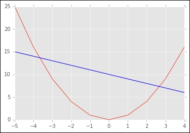
The parabola is a convex function because the values between x1 and x2 (the two points where the blue line intersects with the parabola) are always below the blue line representing α(F(x1))+(1-α) (F(x2)). As you can see, the parabola also has a global minimum between these two points.

When we are dealing with matrices such as the Hessian referenced previously, this condition is fulfilled by each element of the matrix being ≥ 0, a property known as positive semidefinite, meaning any vector multiplied by this matrix on either side (xTHx) yields a value ≥ 0. This means the function has a global minimum, and if our solution converges to a set of coefficients, we can be guaranteed that they represent the best parameters for the model, not a local minimum.

We noted previously that we could potentially offset imbalanced distribution of classes in our data by reweighting individual points during training. In the formulas for either SGD or IRLS, we could apply a weight wi for each data point, increasing or decreasing its relative contribution to the value of the likelihood and the updates made during each iteration of the optimization algorithm.

Now that we have described how to obtain the optimal parameters of the logistic regression model, let us return to our example and apply these methods to our data.