
The trend line is a common feature of many business analyses. How much do purchases increase when ads are shown more often on a homepage? What is the average rating of videos on social media based on user age? What is the likelihood that a customer will buy a second product from your website if they bought their first more than 6 months ago? These sorts of questions can be answered by drawing a line representing the average change in our response (for example, purchases or ratings) as we vary the input (for example, user age or amount of past purchases) based on historical data, and using it to extrapolate the response for future data (where we only know the input, but not output yet). Calculating this line is termed regression, based on the hypothesis that our observations are scattered around the true relationship between the two variables, and on average future observations will regress (approach) the trend line between input and output.
Several complexities complicate this analysis in practice. First, the relationships we fit usually involve not one, but several inputs. We can no longer draw a two dimensional line to represent this multi-variate relationship, and so must increasingly rely on more advanced computational methods to calculate this trend in a high-dimensional space. Secondly, the trend we are trying to calculate may not even be a straight line – it could be a curve, a wave, or even more complex patterns. We may also have more variables than we need, and need to decide which, if any, are relevant for the problem at hand. Finally, we need to determine not just the trend that best fits the data we have, but also generalizes best to new data.
In this chapter we will learn:
- How to prepare data for a regression problem
- How to choose between linear and nonlinear methods for a given problem
- How to perform variable selection and assess over-fitting
Ordinary Least Squares (OLS).
We will start with the simplest model of linear regression, where we will simply try to fit the best straight line through the data points we have available. Recall that the formula for linear regression is:
Where y is a vector of n responses we are trying to predict, X is a vector of our input variable also of length n, and β is the slope response (how much the response y increases for each 1-unit increase in the value of X). However, we rarely have only a single input; rather, X will represent a set of input variables, and the response y is a linear combination of these inputs. In this case, known as multiple linear regression, X is a matrix of n rows (observations) and m columns (features), and β is a vector set of slopes or coefficients which, when multiplied by the features, gives the output. In essence, it is just the trend line incorporating many inputs, but will also allow us to compare the magnitude effect of different inputs on the outcome. When we are trying to fit a model using multiple linear regression, we also assume that the response incorporates a white noise error term ε, which is a normal distribution with mean 0 and a constant variance for all data points.
To solve for the coefficients β in this model, we can perform the following calculations:

The value of β is known the ordinary least squares estimate of the coefficients. The result will be a vector of coefficients β for the input variables. We make the following assumptions about the data:
- We assume the input variables (X) are accurately measured (there is no error in the values we are given). If they were not, and incorporated error, then they represent random variables, and we would need to incorporate this error in our estimate of the response in order to be accurate.
- The response is a linear combination of the input variables – in other words, we need to be able to fit a straight line through the response. As we will see later in this chapter, we can frequently perform transformations to change nonlinear data into a linear form to satisfy this assumption.
- The residual (the difference between the fitted and actual response) of the response y is assumed to have constant variance over the range of its values. If this is not the case (for example, if smaller values of y have smaller errors than larger values), then it suggests we are not appropriately incorporating a source of error in our model, because the only variation left after we account for the predictors X should be the error term ε. As previously mentioned, this error term ε should have constant variance, meaning the fit should have constant residual variance.
- The residuals are assumed to be un-correlated based on the value of the predictors X. This is important because we assume we are trying to fit a line that goes through the average of the response data points at each predictor value, which would be accurate if we assume that the residual error is randomly distributed about 0. If the residuals are correlated with the value of a predictor, then the line that accurately fits the data may not go through the average, but rather be determined by the underlying correlation in the data. For example, if we are looking at time-series data, days of the week may have more correlated error at a 7-day pattern, meaning that our model should fit this periodicity rather than trying to simply draw a line through the data points for all days together.
- The predictors are assumed not to be collinear (correlated with one another). If two predictors are identical, then they cancel each other out when we make a linear combination of the input matrix X. As we can see in the derivation of β above, to calculate the coefficients we need to take an inverse. If columns in the matrix exactly cancel each other out, then this matrix (XTX)-1 is rank deficient and has no inverse. Recall that if a matrix is full rank, its columns (rows) cannot be represented by a linear combination of the other columns (rows). A rank-deficient does not have an inverse because if we attempt to solve the linear system represented by:
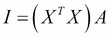
Where A is the inverse we are trying to solve and I is the identity matrix, we will end up with columns in the solution the exactly cancel each-other, meaning any set of coefficients will solve the equation and we cannot have a unique solution.
Why does the OLS formula for β represent the best estimate of the coefficients? The reason is that this value minimizes the squared error:

While a derivation of this fact is outside the scope of this text, this result is known as the Gauss Markov Theorem, and states that the OLS estimate is the Best Linear Unbiased Estimator (BLUE) of the coefficients β. Recall that when we are estimating these coefficients, we are doing so under the assumption that our calculations have some error, and deviate from the real (unseen) values. The BLUE is then the set of coefficients β that have the smallest mean error from these real values. For more details, we refer the reader to more comprehensive texts (Greene, William H. Econometric analysis. Pearson Education India, 2003; Plackett, Ronald L. "Some theorems in least squares." Biometrika 37.1/2 (1950): 149-157).
Depending upon the problem and dataset, we can relax many of the assumptions described above using alternative methods that are extensions of the basic linear model. Before we explore these alternatives, however, let us start with a practical example. The data we will be using for this exercise is a set of news articles from the website http://mashable.com/. (Fernandes, Kelwin, Pedro Vinagre, and Paulo Cortez. "A Proactive Intelligent Decision Support System for Predicting the Popularity of Online News." Progress in Artificial Intelligence. Springer International Publishing, 2015. 535-546.). Each article has been annotated using a number of features such as its number of words and what day it was posted - a complete list appears in the data file associated with this exercise. The task is to predict the popularity (the share column in the dataset) using these other features. In the process of fitting this first model, we will examine some of the common feature preparation tasks that arise in such analyses.
Let us start by taking a look at the data by typing the following commands:
>>> news = pd.read_csv('OnlineNewsPopularity.csv',sep=',')
>>> news.columns
Which gives the output:
Index(['url', ' timedelta', ' n_tokens_title', ' n_tokens_content', ' n_unique_tokens', ' n_non_stop_words', ' n_non_stop_unique_tokens', ' num_hrefs', ' num_self_hrefs', ' num_imgs', ' num_videos', ' average_token_length', ' num_keywords', ' data_channel_is_lifestyle', ' data_channel_is_entertainment', ' data_channel_is_bus', ' data_channel_is_socmed', ' data_channel_is_tech', ' data_channel_is_world', ' kw_min_min', ' kw_max_min', ' kw_avg_min', ' kw_min_max', ' kw_max_max', ' kw_avg_max', ' kw_min_avg', ' kw_max_avg', ' kw_avg_avg', ' self_reference_min_shares', ' self_reference_max_shares', ' self_reference_avg_sharess', ' weekday_is_monday', ' weekday_is_tuesday', ' weekday_is_wednesday', ' weekday_is_thursday', ' weekday_is_friday', ' weekday_is_saturday', ' weekday_is_sunday', ' is_weekend', ' LDA_00', ' LDA_01', ' LDA_02', ' LDA_03', ' LDA_04', ' global_subjectivity', ' global_sentiment_polarity', ' global_rate_positive_words', ' global_rate_negative_words', ' rate_positive_words', ' rate_negative_words', ' avg_positive_polarity', ' min_positive_polarity', ' max_positive_polarity', ' avg_negative_polarity', ' min_negative_polarity', ' max_negative_polarity', ' title_subjectivity', ' title_sentiment_polarity', ' abs_title_subjectivity', ' abs_title_sentiment_polarity', ' shares'], dtype='object')
If you look carefully, you will realize that all the column names have a leading whitespace; you probably would have found out anyway the first time you try to extract one of the columns by using the name as an index. The first step of our data preparation is to fix this formatting using the following code to strip whitespace from every column name:
>>> news.columns = [ x.strip() for x in news.columns]
Now that we have correctly formatted the column headers, let us examine the distribution of the data using the describe() command as we have seen in previous chapters:

As you scroll from left to right along the columns, you will notice that the range of the values in each column is very different. Some columns have maximum values in the hundreds or thousands, while others are strictly between 0 and 1. In particular, the value that we are trying to predict, shares, has a very wide distribution, as we can see if we plot the distribution using the following command:
>>> news['shares'].plot(kind='hist',bins=100)

Why is this distribution a problem? Recall that conceptually, when we fit a line through a dataset, we are finding the solution to the equation:
Where y is a response variable (such as shares), and β is the vector slopes by which we increase/decrease the value of the response for a 1-unit change in a column of X. If our response is logarithmically distributed, then the coefficients will be biased to accommodate extremely large points in order to minimize the total error of the fit given by:

To reduce this effect, we can logarithmically transform the response variable, which as you can see through the following code makes a distribution that looks much more like a normal curve:
>>> news['shares'].map( lambda x: np.log10(x) ).plot(kind='hist',bins=100)

This same rule of thumb holds true for our predictor variables, X. If some predictors are much larger than others, the solution of our equation will mainly emphasize those with the largest range, as they will contribute most to the overall error. In this example, we can systemically scale all of our variables using a logarithmic transformation. First, we remove all uninformative columns, such as the URL, which simply gives website location for the article.
>>> news_trimmed_features = news.ix[:,'timedelta':'shares']
Note
Note that in Chapter 6, Words and Pixels – Working with Unstructured Data we will explore potential ways to utilize information in textual data such as the url, but for now we will simply discard it.
Then, we identify the variables we wish to transform (here an easy rule of thumb is that their max, given by the 8th row (index 7) of the describe() data frame is > 1, indicating that they are not in the range 0 to 1) and use the following code to apply the logarithmic transform. Note that we add the number 1 to each logarithmically transformed variable so that we avoid errors for taking the logarithm of 0.
>>> log_values = list(news_trimmed_features.columns[news_trimmed_features.describe().reset_index().loc[7][1:]>1])
>>> for l in log_values:
…    news_trimmed_features[l] = np.log10(news_trimmed_features[l]+1)
Using the describe() command again confirms that the columns now have comparable distributions:

We also need to remove infinite or nonexistent values from the dataset. We first convert infinite values to the placeholder 'not a number', or NaN, using the following:
>>> news_trimmed_features = news_trimmed_features.replace([np.inf, -np.inf], np.nan)
We then use the fill function to substitute the NaN placeholder with the proceeding value in the column (we could also have specified a fixed value, or used the preceding value in the column) using the following:
>>> news_trimmed_features = news_trimmed_features.fillna(method='pad')
Now we can split the data into the response variable ('shares') and the features (all columns from 'timedelta' to 'abs_title_sentiment_polarity'), which we will use as inputs in the regression models described later using the commands:
>>> news_response = news_trimmed_features['shares']
>>> news_trimmed_features = news_trimmed_features.ix[:,'timedelta':'abs_title_sentiment_polarity']
Let us now also take another look at variables that we did not transform logarithmically. If you try to fit a linear model using the dataset at this point, you will find that the slopes for many of these are extremely large or small. This can be explained by looking at what the remaining variables represent. For example, one set of columns which we did not logarithmically transform encodes a 0/1 value for whether a news article was published on a given day of the week. Another (annotated LDA) gives a 0/1 indicator for whether an article was tagged with a particular algorithmically-defined topic (we will cover this algorithm, known as Latent Dirichlet Allocation, in more detail in Chapter 6, Words and Pixels – Working with Unstructured Data). In both cases, any row in the dataset must have the value 1 in one of the columns of these features (for example, the day of week has to take one of the seven potential values). Why is this a problem?
Recall that in most linear fits, we have both a slope and an intercept, which is the offset of the line vertically from the origin (0, 0) of the x-y plane. In a linear model with many variables, we represent this multi-dimensional intercept by a column of all 1 in the feature matrix X, which will be added by default in many model-fitting libraries. This means that a set of columns (for example, the days of the week), since they are independent, could form a linear combination that exactly equals the intercept column, making it impossible to find a unique solution for the slopes β. This is the same issue as the last assumption of linear regression we discussed previously, in which the matrix (XTX) is not invertible, and thus we cannot obtain a numerically stable solution for the coefficients. This instability results in the unreasonably large coefficient values you will observe if you were to fit a regression model on this dataset. It is for this reason that we either need to leave out the intercept column (an option you usually need to specify in a modeling library), or leave out one of the columns for these binary variables. Here we will do the second, dropping one column from each set of binary features using the following code:
>>> news_trimmed_features = news_trimmed_features.drop('weekday_is_sunday',1)
>>> news_trimmed_features = news_trimmed_features.drop('LDA_00',1)
Now that we have taken care of these feature engineering concerns, we are ready to fit a regression model to our data.
Now that we are ready to fit a regression model to our data, it is important to clarify the goal of our analysis. As we discussed briefly in Chapter 1, From Data to Decisions – Getting Started with Analytic Applications, the goals of modeling can be either a) to predict a future response given historical data, or b) infer the statistical significance and effect of a given variable on an outcome.
In the first scenario, we will choose a subset of data to train our model, and then evaluate the goodness of fit of the linear model on an independent data set not used to derive the model parameters. In this case, we want to validate that the trends represented by the model generalize beyond a particular set of data points. While the coefficient outputs of the linear model are interpretable, we are still more concerned in this scenario about whether we can accurately predict future responses rather than the meaning of the coefficients.
In the second scenario, we may not use a test data set at all for validation, and instead fit a linear model using all of our data. In this case, we are more interested in the coefficients of the model and whether they are statistically significant. In this scenario, we are also frequently interested in comparing models with more or fewer coefficients to determine the most important parameters that predict an outcome.
We will return to this second case, but for now let us continue under the assumption that we are trying to predict future data. To obtain test and validation data, we use the following commands to split the response and predictor data into 60% training and 40% test splits:
>>> from sklearn import cross_validation
>>> news_features_train, news_features_test, news_shares_train, news_shares_test =
>>> cross_validation.train_test_split(news_trimmed_features, news_response, test_size=0.4, random_state=0)
We use the 'random state' argument to set a fixed outcome for this randomization, so that we can reproduce the same train/test split if we want to rerun the analysis at later date. With these training and test sets we can then fit the model and compare the predicted and observed values visually using the following code:
>>> from sklearn import linear_model
>>> lmodel = linear_model.LinearRegression().fit(news_features_train, news_shares_train)
>>> plt.scatter(news_shares_train,lmodel.predict(news_features_train),color='black')
>>> plt.xlabel('Observed')
>>> plt.ylabel('Predicted')
Which gives the following plot:

Similarly, we can look at the performance of the model on the test data set using the commands:
>>> plt.scatter(news_shares_test,lmodel.predict(news_features_test),color='red')
>>> plt.xlabel('Observed')
>>> plt.ylabel('Predicted')
Which gives the plot:

The visual similarities are confirmed by looking at the coefficient of variation, or 'R-squared' value. This is a metric often used in regression problems, which defines how much of the variation in the response is explained by the variation in the predictors according to the model. It is computed as:

Where Cov and Var are the Covariance and Variance (respectively) of the two variables (the observed response y, and the predicted response given by yβ). A perfect score is 1 (a straight line), while 0 represents no correlation between a predicted and observed value (an example would be a spherical cloud of points). Using scikit learn, we can obtain the R2 value using the score() method of the linear model, with arguments the features and response variable. Running the following for our data:
>>> lmodel.score(news_features_train, news_shares_train)
>>> lmodel.score(news_features_test, news_shares_test)
We get a value of 0.129 for the training data and 0.109 for the test set. Thus, we see that while there is some relationship between the predicted and observed response captured in the news article data, though we have room for improvement.
In addition to looking for overall performance, we may also be interested in which variables from our inputs are most important in the model. We can sort the coefficients of the model by their absolute magnitude to analyse this using the following code to obtain the sorted positions of the coefficients, and reorder the column names using this new index:
>>> ix = np.argsort(abs(lmodel.coef_))[::-1][:]
>>> news_trimmed_features.columns[ix]
This gives the following output:
Index([u'n_unique_tokens', u'n_non_stop_unique_tokens', u'n_non_stop_words', u'kw_avg_avg', u'global_rate_positive_words', u'self_reference_avg_sharess', u'global_subjectivity', u'LDA_02', u'num_keywords', u'self_reference_max_shares', u'n_tokens_content', u'LDA_03', u'LDA_01', u'data_channel_is_entertainment', u'num_hrefs', u'num_self_hrefs', u'global_sentiment_polarity', u'kw_max_max', u'is_weekend', u'rate_positive_words', u'LDA_04', u'average_token_length', u'min_positive_polarity', u'data_channel_is_bus', u'data_channel_is_world', u'num_videos', u'global_rate_negative_words', u'data_channel_is_lifestyle', u'num_imgs', u'avg_positive_polarity', u'abs_title_subjectivity', u'data_channel_is_socmed', u'n_tokens_title', u'kw_max_avg', u'self_reference_min_shares', u'rate_negative_words', u'title_sentiment_polarity', u'weekday_is_tuesday', u'min_negative_polarity', u'weekday_is_wednesday', u'max_positive_polarity', u'title_subjectivity', u'weekday_is_thursday', u'data_channel_is_tech', u'kw_min_avg', u'kw_min_max', u'kw_avg_max', u'timedelta', u'kw_avg_min', u'kw_max_min', u'max_negative_polarity', u'kw_min_min', u'avg_negative_polarity', u'weekday_is_saturday', u'weekday_is_friday', u'weekday_is_monday', u'abs_title_sentiment_polarity'], dtype='object')
You will notice that there is no information on the variance of the parameter values. In other words, we do not know the confidence interval for a given coefficient value, nor whether it is statistically significant. In fact, the scikit-learn regression method does not calculate statistical significance measurements, and for this sort of inference analysis—the second kind of regression analysis discussed previously and in Chapter 1, From Data to Decisions – Getting Started with Analytic Applications—we will turn to a second Python library, statsmodels (http://statsmodels.sourceforge.net/).
After installing the statsmodels library, we can perform the same linear model analysis as previously, using all of the data rather than a train/test split. With statsmodels, we can use two different methods to fit the linear model, api and formula.api, which we import using the following commands:
>>> import statsmodels
>>> import statsmodels.api as sm
>>> import statsmodels.formula.api as smf
The api methods first resembles the scikit-learn function call, except we get a lot more detailed output about the statistical significance of the model after running the following:
>>> results = sm.OLS(news_response, news_trimmed_features).fit()
>>> results.summary()
Which gives the following output:
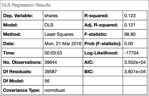
What do all these parameters mean? The number of observations and number of dependent variables are probably obvious, but the others we have not seen before. Briefly, their names and interpretation are:
- Df model: This is the number of independent elements in the model parameters. We have 57 columns; once we know the value of 56 of them, the last is fixed by the need to minimize the remaining error, so there are only 56 degrees of freedom overall.
- Df residuals: This is the number of independent pieces of information in the error estimates of the model. Recall that we obtain the errors by
y-X.We only have up tomindependent columns inX, wheremis the number of predictors. So our estimate of the error hasn-1independent elements from the data itself, from which we subtract anothermwhich is determined by the inputs, giving usn-m-1. - Covariance type: This is the kind of covariance used in the model; here we just use white noise (a mean
0, normally distributed error), but we could just as easily have specified a particular structure that would accommodate, for example, a case where the error is correlated with the magnitude of the response. - Adj. R-squared: If we include more variables in a model, we can start to increase the R2 by simply having more degrees of freedom with which to fit the data. If we wish to fairly compare the R2 for models with different numbers of parameters, then we can adjust the R2 calculation with the following formula:

Using this formula, for models with larger numbers of parameters, we penalize the R2 by the amount of error in the fit.
- F-statistics: This measure is used to compare (through a Chi-squared distribution) that any of the regression coefficients are statistically different than
0. - Prob (F-statistic): This is the p-value (from the F-statistic) that the null hypothesis (that the coefficients are
0and the fit is no better than the intercept-only model) is true. - Log-likelihood: Recall that we assume the error of the residuals in the linear model is normally distributed. Therefore, to determine how well our result fits this assumption, we can compute the likelihood function:

Where σ is the standard deviation of the residuals and μ is the mean of the residuals (which we expect be very near 0 based on the linear regression assumptions above). Because the log of a product is a sum, which is easier to work with numerically, we usually take the logarithm of this value, expressed as:

While this value is not very useful on its own, it can help us compare two models (for example with different numbers of coefficients). Better goodness of fit is represented by a larger log likelihood, or a lower negative log likelihood.
- AIC/BIC: AIC and BIC are abbreviations for the Akaike Information Criterion and Bayes Information Criterion. These are two statistics that help to compare models with different numbers of coefficients, thus giving a sense of the benefit of greater model complexity from adding more features. AIC is given by:
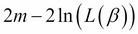
Where m is the number of coefficients in the model and L is the likelihood, as described previously. Better goodness of fit is represented by lower AIC. Thus, increasing the number of parameters penalizes the model, while improving the likelihood that it decreases the AIC. BIC is similar, but uses the formula:
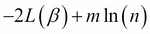
Where n is the number of data points in the model. For a fuller comparison of AIC and BIC, please see (Burnham, Kenneth P., and David R. Anderson. Model selection and multimodel inference: a practical information-theoretic approach. Springer Science & Business Media, 2003).
Along with these, we also receive an output of the statistical significance of each coefficient, as judged by a t-test of its standard error:

We also receive a final block of statistics:

Most of these are outside the scope of this volume, but the Durbin-Watson (DW) statistic will be important later, when we discuss dealing with time series data. The DW statistic is given by:

Where e are the residuals (here y-Xβ for the linear model). In essence, this statistic asks whether the residuals are positively or negatively correlated. If its value is >2, this suggests a positive correlation. Values between 1 and 2 indicate little to correlation, with 2 indicating no correlation. Values less than 1 represent negative correlation between successive residuals. For more detail please see (Chatterjee, Samprit, and Jeffrey S. Simonoff. Handbook of regression analysis. Vol. 5. John Wiley & Sons, 2013).
We could also have fit the model using the formula.api commands, by constructing a string from the input data representing the formula for the linear model. We generate the formula using the following code:
>>> model_formula = news_response.name+" ~ "+" + ".join(news_trimmed_features.columns)
You can print this formula to the console to verify it gives the correct output:
shares ~ timedelta + n_tokens_title + n_tokens_content + n_unique_tokens + n_non_stop_words + n_non_stop_unique_tokens + num_hrefs + num_self_hrefs + num_imgs + num_videos + average_token_length + num_keywords + data_channel_is_lifestyle + data_channel_is_entertainment + data_channel_is_bus + data_channel_is_socmed + data_channel_is_tech + data_channel_is_world + kw_min_min + kw_max_min + kw_avg_min + kw_min_max + kw_max_max + kw_avg_max + kw_min_avg + kw_max_avg + kw_avg_avg + self_reference_min_shares + self_reference_max_shares + self_reference_avg_sharess + weekday_is_monday + weekday_is_tuesday + weekday_is_wednesday + weekday_is_thursday + weekday_is_friday + weekday_is_saturday + is_weekend + LDA_01 + LDA_02 + LDA_03 + LDA_04 + global_subjectivity + global_sentiment_polarity + global_rate_positive_words + global_rate_negative_words + rate_positive_words + rate_negative_words + avg_positive_polarity + min_positive_polarity + max_positive_polarity + avg_negative_polarity + min_negative_polarity + max_negative_polarity + title_subjectivity + title_sentiment_polarity + abs_title_subjectivity + abs_title_sentiment_polarity
We can then use this formula to fit the full pandas dataframe containing both the response and the input variables, by concatenating the response and feature variables along their columns (axis 1) and calling the ols method of the formula API we imported previously:
>>> news_all_data = pd.concat([news_trimmed_features,news_response],axis=1)
>>> results = smf.ols(formula=model_formula,data=news_all_data).fit()
In this example, it seems reasonable to assume that the residuals in the model we fit for popularity as a function of new article features are independent. For other cases, we might make multiple observations on the same set of inputs (such as when a given customer appears more than once in a dataset), and this data may be correlated with time (as when records of a single customer are more likely to be correlated when they appear closer together in time). Both scenarios violate our assumptions of independence among the residuals in a model. In the following sections we will introduce three methods to deal with these cases.
In our next set of exercises we will use an example of student grades in a math course in several schools recorded over three terms, expressed by the symbols (G1-3) (Cortez, Paulo, and Alice Maria Gonçalves Silva. "Using data mining to predict secondary school student performance." (2008)). It might be expected that there is a correlation between the school in which the student is enrolled and their math grades each term, and we do see some evidence of this when we plot the data using the following commands:
>>> students = pd.read_csv('student-mat.csv',sep=';')
>>> students.boxplot(by='school',column=['G1','G2','G3'])

We can see that there is some correlation between a decline in math grades in terms 2 and 3, and the school. If we want to estimate the effect of other variables on student grades, then we want to account for this correlation. How we do so depends upon what our objective is. If we want to simply have an accurate estimate of the coefficients β of the model at the population level, without being able to predict individual students' responses with our model, we can use the Generalize Estimating Equations (GEE) (Liang, Kung-Yee, and Scott L. Zeger. "Longitudinal data analysis using generalized linear models." Biometrika 73.1 (1986): 13-22). The motivating idea of the GEE is that we treat this correlation between school and grade as an additional parameter (which we estimate by performing a linear regression on the data and calculating the residuals) in the model. By doing so, we account for the effect of this correlation on the coefficient estimate, and thus obtain a better estimate of their value. However, we still usually assume that the responses within a group are exchangeable (in other words, the order does not matter), which is not the case with clustered data that might have a time-dependent component.
Unlike the linear model, GEE parameter estimates are obtained through nonlinear optimization of the objective function U(β), using the following formula:

Where μk is the mean response of a group k (such as a school, in our example), Vk is the variance matrix giving the correlation between residuals for members of the group k and Yk- μk is the vector of residuals within this group. This is usually solved using the Newton-Raphson equation, which we will look at in more detail in Chapter 5, Putting Data in its Place – Classification Methods and Analysis. Conceptually, we can estimate the variance matrix V using the residuals from a regression, and optimize the formula above until convergence. Thus, by optimizing both the correlation structure between grouped data samples given by V along with the coefficients β, we have effectively obtained an estimate β independent of V.
To apply this method to our data, we can again create the model string using the following command:
>>> model_formula = "G3 ~ "+" + ".join(students.columns[1:len(students.columns)-3])
We can then run the GEE using the school as the grouping variable:
>>> results = smf.gee(model_formula,"school",data=students).fit()
>>> results.summary()
However, in some cases we would instead like to obtain an estimate of individual, not population-level, responses, even with the kind of group correlations we discussed previously. In this scenario, we could instead use mixed effects models.
Recall that in the linear models we have fitted in this chapter, we assume the response is modeled as:
Where ε is an error term. However, when we have correlation between data points belonging to a group, we can also use a model of the form:
Where Z and u are group-level variables and coefficients, respectively. The coefficient u has a mean 0 and a variance structure that needs to be specified. It could be uncorrelated between groups, for example, or have a more complex covariance relationship where certain groups are correlated with one another more strongly than others. Unlike the GEE model, we are not attempting to simply estimate the group level effect of the coefficients (after factoring out the effect of group membership), but within-group coefficients that control for the effect of belonging to a particular group. The name of mixed effects models comes from the fact that the variables β are fixed effects whose value is exactly known, while u are random effects, where the value u represents an observation of a group level coefficient which is a random variable. The coefficients u could either be a set of group-level intercepts (random intercepts model), or combined with group-level slopes (random slopes model). Groups may even be nested within one another (hierarchical mixed effects models), such as if town-level groups capture one kind of correlated variation, while state-level groups capture another. A full discussion of the many variations of mixed effects models is outside the scope of this book, but we refer the interested reader to references such as (West, Brady T., Kathleen B. Welch, and Andrzej T. Galecki. Linear mixed models: a practical guide using statistical software. CRC Press, 2014; Stroup, Walter W. Generalized linear mixed models: modern concepts, methods and applications. CRC press, 2012). As with GEE, we can fit this model similar to the linear model by including a group-level variable using the following commands:
>>> results = smf.mixedlm(model_formula,groups="school",data=students).fit()
>>> results.summary()
The last category of model assumptions that we will consider are where clustered data is temporally correlated, for example if a given customer has periodic buying activity based on the day of the week. While GEE and mixed effects models generally deal with data in which the inter-group correlations are exchangeable (the order does not matter), in time series data, the order is important for the interpretation of the data. If we assume exchangeability, then we may incorrectly estimate the error in our model, since we will assume the best fit goes through the middle of the data in a given group, rather than following the correlation structure of repeated measurements in a time series.
A particularly flexible model for time series data uses a formula known as the Kalman filter. Superficially, the Kalman filter resembles the equation for mixed effects models; consider an observation that at a given point in time has an unobserved state which we want to infer in the model (such as whether a given stock is increasing or decreasing in price), which is obscured by noise (such as market variation in stock price). The state of the data point is given by:
Where F represents the matrix of transition probabilities between states, xt-1 is the state at the last time step, wt is noise, and Bt and ut represent regression variables that could incorporate, for example, seasonal effects. In this case, u would be a binary indicator of a season or time of day, and β the amount we should add or subtract from x based on this indicator. The state x is used to predict the observed response using:
Where xt is the state from the previous equation, H is a set of coefficients for each underlying state, and vt is noise. The Kalman filter uses the observations at time t-1 to update our estimates of both the underlying state x and the response y at time t.
The family of equations given previously is also known by the more general term "Structural Time Series Equations". For the derivations of the update equations and further details on "Structural Time Series Models", we refer the reader to more advanced references (Simon, Dan. Optimal state estimation: Kalman, H infinity, and nonlinear approaches. John Wiley & Sons, 2006; Harvey, Andrew C. Forecasting, structural time series models and the Kalman filter. Cambridge University Press, 1990).
In the statsmodels package, the Kalman filter is used in auto-regressive moving average (ARMA) models, which are fit with the following command:
>>> statsmodels.tsa.arima_model.ARMA()
In most of the preceding examples, we assume that the response variable may be modeled as a linear combination of the responses. However, we can often relax this assumption by fitting a generalized linear model. Instead of the formula:
We substitute a link function (G) that transforms the nonlinear output into a linear response:
Examples of link functions include:
- Logit: This
linkfunction maps the responses in the range0to1to a linear scale using the function Xβ=ln(y/1-y), where y is usually a probability between0and1. Thislinkfunction is used in logistic and multinomial regression, covered in Chapter 5, Putting Data in its Place – Classification Methods and Analysis. - Poisson: This
linkfunction maps count data to a linear scale using the relationship Xβ=ln(y), where y is count data. - Exponential: This
linkfunction maps data from an exponential scale to a linear one with the formula Xβ=y-1.
While these sorts of transformations make it possible to transform many nonlinear problems into linear ones, they also make it more difficult to estimate parameters of the model. Indeed, the matrix algebra used to derive the coefficients for simple linear regression do not apply, and the equations do not have any closed solution we could represent by a single step or calculation. Instead, we need iterative update equations such as those used for GEE and mixed effects models. We will cover these sorts of methods in more detail in Chapter 5, Putting Data in its Place – Classification Methods and Analysis.
Now we have now covered some of the diverse cases of fitting models to data that violate the linear regression assumptions in order to correctly interpret coefficients. Let us return now to the task of trying to improve the predictive performance of our linear model by selecting a subset of variables in the hope of removing correlated inputs and reducing over-fitting, an approach known as regularization.
After observing that the performance of our linear model is not optimal, one relevant question is whether all of the features in this model are necessary, or whether the coefficients we have estimated are suboptimal. For instance, two columns may be highly correlated with one another, meaning that the matrix XTX can be rank-deficient and thus not invertible, leading to numerical instability in calculating the coefficients. Alternatively, we may have included enough input variables to make an excellent fit on the training data, but this fit may not generalize to the test data as it precisely captures nuanced patterns present only in the training data. The high number of variables gives us great flexibility to make the predicted responses exactly match the observed responses in the training set, leading to overfitting. In both cases, it may be helpful to apply regularization to the model. Using regularization, we try to apply a penalty to the magnitude and/or number of coefficients, in order to control for over-fitting and multicollinearity. For regression models, two of the most popular forms of regularization are Ridge and Lasso Regression.
In Ridge Regression, we want to constrain the coefficient magnitude to a reasonable level, which is accomplished by applying a squared penalty to the size of the coefficients in the loss function equation:

In other words, by applying the penalty α to the sum of squares of the coefficients, we constrain the model not only to approximate y as well as possible, using the slopes β multiplied by the features, but also constrain the size of the coefficients β. The effect of this penalty is controlled by the weighting factor α. When alpha is 0, the model is just normal linear regression. Models with α > 0 increasingly penalizes large β values. How can we choose the right value for α? The scikit-learn library offers a helpful cross-validation function that can find the optimal value for α on the training set using the following commands:
>>> lmodel_ridge = linear_model.RidgeCV().fit(news_features_train, news_shares_train)
>>> lmodel_ridge.alpha_
Which gives the optimal α value as 0.100.
However, making this change does not seem to influence predictive accuracy on the test set when we evaluate the new R2 value using the following commands:
>>> lmodel_ridge.score(news_features_test, news_shares_test)
In fact, we obtain the same result as the original linear model, which gave a test set R2 of 0.109.
Another method of regularization is referred to as Lasso, where we minimize the following equation. It is similar to the Ridge Regression formula above, except that the squared penalty on the values of β have been replaced with an absolute value term.

This absolute value penalty has the practical effect that many of the slopes are optimized to be zero. This could be useful if we have many inputs and wish to select only the most important to try and derive insights. It may also help in cases where two variables are closely correlated with one another, and we will select one to include in the model. Like Ridge Regression, we can find the optimal value of α using the following cross validation commands:
>>> lmodel_lasso = linear_model.LassoCV(max_iter=10000).fit(news_features_train, news_shares_train)
>>> lmodel_lasso.alpha_
Which suggests an optimal α value of 6.25e-5.
In this case, there does not seem to be much value in applying this kind of penalization to the model, as the optimal α is near zero. Taken together, the analyses above suggest that modifying the coefficients themselves is not helping our model.
What might help us decide whether we would use Ridge or Lasso, besides the improvement in goodness of fit? One tradeoff is that while Lasso may generate a sparser model (more coefficients set to 0), the values of the resulting coefficients are hard to interpret. Given two highly correlated variables, Lasso will select one, while shrinking the other to 0, meaning with some modification to the underlying data (and thus bias to select one of these variables) we might have selected a different variable into the model. While Ridge regression does not suffer from this problem, the lack of sparsity may make it harder to interpret the outputs as well, as it does not tend to remove variables from the model.
A balance between these two choices is provided by Elastic Net Regression (Zou, Hui, and Trevor Hastie. "Regularization and variable selection via the elastic net." Journal of the Royal Statistical Society: Series B (Statistical Methodology) 67.2 (2005): 301-320.). In Elastic Net, our penalty term becomes a blend of Ridge and Lasso, with the optimal β minimizing:

Because of this modification, Elastic Net can select groups of correlated variables, while still shrinking many to zero. Like Ridge and Lasso, Elastic Net has a CV function to choose the optimal value of the two penalty terms α using:
>>> from sklearn.linear_model import ElasticNetCV
>>> lmodel_enet = ElasticNetCV().fit(news_features_train, news_shares_train)
>>> lmodel_enet.score(news_features_test, news_shares_test)
However, this still is not significantly improving the performance of our model, as the test R2 is still unmoved from our original least squares regression. It may be the response is not captured well by a linear trend involving a combination of the inputs. There may be interactions between features that are not represented by coefficients of any single variable, and some variables might have nonlinear responses, such as:
- Nonlinear trends, such as a logarithmic increase in the response for a linear increase in the predictor
- Non-monotonic (increasing or decreasing) functions such as a parabola, with a lower response in the middle of the range of predictor values and higher values at the minimum and maximum
- More complex multi-modal responses, such as cubic polynomials
While we could attempt to use generalized linear models, as described above, to capture these patterns, in large datasets we may struggle to find a transformation that effectively captures all these possibilities. We might also start constructing "interaction features" by, for example, multiplying each of our input variables to generate N(N-1)/2 additional variables (for the pairwise products between all input variables). While this approach, sometimes called "polynomial expansion," can sometimes capture nonlinear relationships missed in the original model, with larger feature sets this can ultimately become unwieldy. Instead, we might try to explore methods that can efficiently explore the space of possible variable interactions.