
Imagine a situation where we have a dataset from a supermarket store about the gender of the customer and whether that person bought a particular product or not. We are interested in finding the chances of a customer buying that particular product, given their gender. What comes to mind when someone poses this question to you? Probability anyone? Odds of success?
What is the probability of a customer buying a product, given he is a male? What is the probability of a customer buying that product, given she is a female? If we know the answers to these questions, we can make a leap towards predicting the chances of a customer buying a product, given their gender.
Let us look at such a dataset. To do so, we write the following code snippet:
import pandas as pd
df=pd.read_csv('E:/Personal/Learning/Predictive Modeling Book/Book Datasets/Logistic Regression/Gender Purchase.csv')
df.head()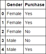
Fig. 6.1: Gender and Purchase dataset
The first column mentions the gender of the customer and the second column mentions whether that particular customer bought the product or not. There are a total of 511 rows in the dataset, as can be found out by typing df.shape.
A contingency table is basically a representation of the frequency of observations falling under various categories of two or more variables. It comes in a matrix form and essentially contains the frequency of occurrences for the combination of categories of two or more variables.
Let us create a contingency table for the dataset we just imported and get a sense of how such a table actually looks. Creating a contingency table in Python is very simple and can be done in a single line using the crosstab method in the pandas library. One can actually create a crosstab object and use it for other purposes such as adding row/column sums. Here, we are creating a contingency table for the Gender and Purchase variables:
contingency_table=pd.crosstab(df['Gender'],df['Purchase'])
contingency_table

Fig. 6.2: Contingency table between Gender and Purchase variables
The interpretation of this table is simple. It implies that there are 106 females who didn't purchase that product, while 159 bought it. Similarly, 125 males didn't buy that particular product, but 121 did. Let us now find the total number of males and females for the purpose of calculating probabilities. The sum can be found out by simple manual addition. However, for the purpose of demonstrating how to do it in Python, let us do it using a code snippet:
contingency_table.sum(axis=1)
contingency_table.sum(axis=0)

Fig. 6.3: Totals across the rows and columns of the contingency table
Rather than calculating numbers, one can calculate the proportions as well. In our case, we will try to calculate the proportion of males and females who purchased and who didn't purchase a particular product. The whole calculation can be done programmatically also using the following code snippet:
contingency_table.astype('float').div(contingency_table.sum(axis=1),axis=0)The result of the snippet looks as follows:

Fig. 6.4: The contingency table for Gender and Purchase in percentage format
Creating a contingency table is a first step towards exploring the data that has a binary outcome variable and categorical predictor variable.
Remember the questions we asked at the beginning of this section? What is the probability of a customer buying a product, given he is a male? What is the probability of a customer buying that product, given she is a female? These questions are the reasons behind something called conditional probability.
Conditional probability basically defines the probability of a certain event happening, given that a certain related event is true or has already happened. Look at the questions above. They perfectly fit the description for conditional probability. The conditional probability of a purchase, given the customer is male, is denoted as follows:
It is calculated by the following formula:

Now, when we know the required numbers and formulae, let us calculate the probabilities we were interested in before:

This concept comes in very handy in understanding many of the predictive models, as it is the building block of many of them.
This is the correct time to introduce a very important concept called odds ratio. The odds ratio is a ratio of odds of success (purchase in this case) for each group (male and female in this case).
Odds of success for a group are defined as the ratio of probability of successes (purchases) to the probability of failures (non-purchases). In our case, the odds of the purchase for the group of males and females can be defined as follows:

Here, Pm=probability of purchase by males and Pf=probability of purchase by females.
For the preceding contingency table given:

As it is obvious from the calculations above, the odds of the success for a particular group can easily be written as follows:

Here, Ns=number of successes in that group and Nf=number of failures in that group.
A few points to be noted about the odds of an event are as follows:
- If the odds of success for a group is more than 1, then it is more likely for that group to be successful. The higher the odds, the better the chances of success.
- If the odds of success is less than 1, then then it is more likely to get a failure. The lower the odds, the higher the chances of failure.
- The odds can range from 0 to infinity.
In our case, the odds of success is greater than 1 for females and less than 1 for males. Thus, we can conclude that females have a better chance of success (purchase), in this case, than males.
One better way to determine which group has better odds of success is by calculating odds ratios for each group. The odds ratio is defined as follows:

In the preceding example we have seen:

Actually,
There are a couple of important things to note about the odds ratio:
- The more the odds ratio, the more the chances of success from that group. In our case, the female group has an odds ratio of 1.54, which means that it is more probable to get success (purchase) from a female customer than a male customer.
- If the odds ratio=1, then there is no association between the two variables. If odds ratio>1, then the event is more likely to happen in Group 1. If the odds ratio<1, then the event is more likely to happen in Group 2.
- Also, the odds ratio for one group can be obtained by taking the reciprocal of the odds ratio of the other group.
If you remember, the equation for a simple linear regression model was as follows:
In this case, Y was a continuous variable whose value can range from –infinity to +infinity. The X was either a continuous or a dummy categorical variable and hence it also ranged from –infinity to +infinity. So, the ranges of variables on both the sides of the equation matched.
However, when we move to logistic regression, the Y variable can take only discrete values, 0 or 1, as the outcome variable is a binary variable. However, predicting 0 or 1 using an equation similar to linear regression is not possible. What if we try to predict the probabilities associated with the two events rather than the binary outcomes? Predicting the probabilities will be feasible as their range spans from 0 to 1.
Earlier, we calculated the conditional probability of a customer purchasing a particular product, given he is male or female. These are the probabilities we are thinking of predicting. In the case demonstrated above, there was only one predictor variable, so it was very easy. However, as the number of predictor variables increase, these conditional probabilities will become more and more difficult to calculate. However, anyways, predicting probability is a better choice than predicting 0 or 1. Hence, for logistic regression, something like the following suits better:
Here P=conditional probability of success/failure given the X variable
Even with this new equation, the problem of non-matching ranges on both the sides of the equation persists. The P ranges from 0 to 1, while X ranges from –infinity to +infinity. What if we replace the P with odds, that is, P/1-P. We have seen earlier that the odds can range from 0 to +infinity. So, the proposed equation becomes:
Where P=conditional probability of success/failure given the X variable
Still the LHS of the equation ranges from 0 to +infinity, while the RHS ranges from –infinity to +infinity. How to get rid of this? We need to transform one side of the equation so that the ranges on both the sides match. What if we take a natural logarithm of the odds (LHS of the equation)? Then, the range on the LHS also becomes –infinity to +infinity.
So, the final equation becomes as follows:
Here, P=conditional probability of success/failure given the X variable.
The term loge(Odds) is called logit.
The transformation can be better understood if we look at the plot of a logarithmic function. For a base greater than 1, the plot of a logarithmic function is shown as follows:

Fig. 6.5: The plot of a logarithmic curve for a base>1
The summary of the ranges of odds and the corresponding ranges of the loge(Odds) can be summarized as follows:
|
Range of Odds |
Range of loge(Odds) |
|---|---|
|
0 to 1 |
-infinity to 0 |
|
1 to +infinity |
0 to +infinity |
The evolution of the transformations that lead from linear to logistic regression can be summarized as follows. The range on the RHS of the equation is always –infinity to +infinity while we transform the LHS to match it:
|
Transformation (LHS) |
Range of LHS |
Range of LHS |
|---|---|---|
|
Y |
Y= 0 or Y= 1 |
Infinity<X<+infinity |
|
P (Probability) |
0<P<1 |
Infinity<X<+infinity |
|
P/1-P (Odds) |
0<P/1-P<+infinity |
Infinity<X<+infinity |
|
log(P/1-P) |
-infinity<log(P/1-P)<+infinity |
Infinity<X<+infinity |
The final equation we have for logistic regression is as follows:

The final equation can be used to calculate the probability, given the value of X, a, and b:
- If a+b*X is very small, then P approaches 0
- If a+b*X is very large, then P approaches 1
- If a+b*X is ), then P=0.5
For a multiple logistic regression, the equation can be written as follows:

If we replace (X1, X2, X3,…,Xn) with Xi' and (b1, b2, b3,----,bn) with bi', the equation can be rewritten as follows:

The variables a and bi are estimated using the Maximum Likelihood Method (MLE).
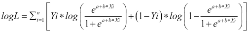
For a multivariate data having multiple variables and n observations, the likelihood (L) or the joint probability is defined as follows:

Here, Pi is the probability associated with the ith observation. When the outcome variable is positive (or 1), we take Pi for multiplying; when it is negative (or 0), we take (1-Pi) for multiplying in the likelihood function:
As we have seen already, the defining equation for logistic regression is as follows:

Also, assume that the output variable is Y1, Y2, Y3,…,Yn, all of which can take the value 0 or 1. For one predictor variable, the best estimate to predict the probability of the success is the mean value of all Yi's:
Here, E[Yi] = Ym is the mean of Yi's.
Hence, the equation above can be rewritten as follows:

Thus, the equation for Likelihood becomes as follows:

Taking log on both the sides:
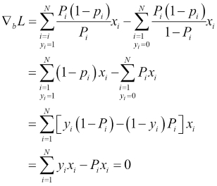
To estimate the MLE of bi's, we equate the derivative of logL to 0:
d(logL)/dXi is the partial derivative of logL with respect to each Xi (variable).
This equation is called the Score function and there would be as many such equations as there are variables in the dataset.
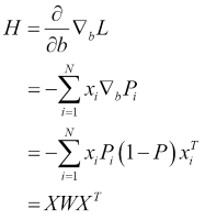
Another related calculation is that of the Fisher Information and it is given as the second derivative of logL:
The Fisher Information is useful because its inverse gives the variance associated with the estimate of the bi. In the case of multiple variables, we will get a covariance matrix. It is also used to decide whether the values found with the help of setting the derivative to 0 were maxima or minima. These many equations will be difficult to solve analytically and there are numerical methods such as Newton-Raphson methods to do the same.
Let us go a little deeper into the mathematics behind calculating the coefficients using the maximum likelihood estimate. The following are the steps in this process:
- Define a function that calculates the probability for each observation, given the data (predictor variables).
- Define a likelihood function that multiplies Pi's and (1-Pi)'s for each observation, depending on whether the outcome is 1 or 0. Calculate the likelihood.
- Use the Newton-Raphson method to calculate the roots. In the Newton-Raphson method, one starts with a value of the root and updates it using the following equation for a number of times until it stops improving:


The derivative of the Log likelihood function is as follows:
The second derivative of the Log likelihood function is as follows:
Partial derivatives have been taken with respect to the variable coefficients.
According to the Newton-Raphson method:

In this case, Newton-Raphson method translates to the following:

Here, W is a diagonal matrix containing the product of probabilities in the diagonal.
Here, we are solving for variable coefficients, that is, a and b. According to the Newton-Raphson method, if we calculate the multiplication above enough number of times, starting with an initial approximate value of variable coefficients (we assume 0 in this case), we will get the optimum values of coefficients. To help better understand the calculation behind the logistic regression, let us implement the mathematics behind the logistic regression using Python code. Let us build the logistic regression model from scratch.
The following are the steps to implement the mathematics behind the logistic regression. Before we start using the in-built methods in Python as a black box to implement logistic regression, let us create a code that can do all the computation and throw up coefficients and likelihoods as the results just the same way as a built in method in Python would. Each of the step has been defined as a separate Python function:
	# Step 1: defining the likelihood function
def likelihood(y,pi):
    import numpy as np
    ll=1
    ll_in=range(1,len(y)+1)
    for i in range(len(y)):
        ll_in[i]=np.where(y[i]==1,pi[i],(1-pi[i]))
        ll=ll*ll_in[i]
    return ll
# Step 2: calculating probability for each observation
def logitprob(X,beta):
    import numpy as np
    rows=np.shape(X)[0]
    cols=np.shape(X)[1]
    pi=range(1,rows+1)
    expon=range(1,rows+1)
    for i in range(rows):
        expon[i]=0
        for j in range(cols):
            ex=X[i][j]*beta[j]
            expon[i]=ex+expon[i]
        with np.errstate(divide='ignore', invalid='ignore'):
            pi[i]=np.exp(expon[i])/(1+np.exp(expon[i]))
    return pi
# Step 3: Calculate the W diagonal matrix
def findW(pi):
    import numpy as np
    W=np.zeros(len(pi)*len(pi)).reshape(len(pi),len(pi))
    for i in range(len(pi)):
        print i
        W[i,i]=pi[i]*(1-pi[i])
        W[i,i].astype(float)
    return W
# Step 4: defining the logistic function
def logistic(X,Y,limit):
    import numpy as np
    from numpy import linalg
    nrow=np.shape(X)[0]
    bias=np.ones(nrow).reshape(nrow,1)
    X_new=np.append(X,bias,axis=1)
    ncol=np.shape(X_new)[1]
    beta=np.zeros(ncol).reshape(ncol,1)
    root_diff=np.array(range(1,ncol+1)).reshape(ncol,1)
    iter_i=10000
    while(iter_i>limit):
        print iter_i, limit
        pi=logitprob(X_new,beta)
        print pi
        W=findW(pi)
        print W
        print X_new
        print (Y-np.transpose(pi))
        print np.array((linalg.inv(np.matrix(np.transpose(X_new))*np.matrix(W)*np.matrix(X_new)))*(np.transpose(np.matrix(X_new))*np.matrix(Y-np.transpose(pi)).transpose()))
        print beta
        print type(np.matrix(np.transpose(Y-np.transpose(pi))))
        print np.matrix(Y-np.transpose(pi)).transpose().shape
        print np.matrix(np.transpose(X_new)).shape
        root_diff=np.array((linalg.inv(np.matrix(np.transpose(X_new))*np.matrix(W)*np.matrix(X_new)))*(np.transpose(np.matrix(X_new))*np.matrix(Y-np.transpose(pi)).transpose()))
        beta=beta+root_diff
        iter_i=np.sum(root_diff*root_diff)
        ll=likelihood(Y,pi)
        print beta
        print beta.shape
    return beta
# Testing the model
import numpy as np
X=np.array(range(10)).reshape(10,1)
Y=[0,0,0,0,1,0,1,0,1,1]
bias=np.ones(10).reshape(10,1)
X_new=np.append(X,bias,axis=1)


# Running logistic Regression using our function
a=logistic(X,Y,0.000000001)
ll=likelihood(Y,logitprob(X,a))
Coefficient of X = 0.66 , Intercept = -3.69
# From stasmodel.api
import statsmodels.api as sm
logit_model=sm.Logit(Y,X_new)
result=logit_model.fit()
print result.summary()
Coefficient of X = 0.66, Intercept = -3.69
Isn't this cool?! We have been able to match the exact values for the variable coefficient and intercept. Run these codes in your Python IDE one by one and see what each snippet throws up as an output. Each of them is a separate function so you will have to give inputs to make them run. Compare it with the calculations performed above and see how the steps in the calculations have been implemented.
In Python, scikit-learn performs these calculations under the hood and throws up the estimates for the coefficients when asked to run a logistic regression.
As with the linear regression, there are various parameters that are thrown up by a logistic regression model, which can be assessed for variable selection and model accuracy.
As in the case of linear regression, here also, we are estimating the values of the coefficients. There is a hypothesis test associated with each estimation. Here, we test the significance of the coefficients bi's:

The Wald statistic is defined as follows:
Here, bim=mean of bi and sd(bi)=standard error in estimation of bi.
The standard error comes from the Fisher Information covariance matrix. The Wald statistic assumes a standard normal distribution and, hence, we can perform a z-test over it. As we will see in the output of a logistic regression, there will be a p-value associated with the estimation of each bi. This p-value comes from this z-test. The smaller the p-value, the more the significance of that variable.
The Likelihood Ratio Test statistic is the ratio of the (null) hypothesized value of the parameter to the MSE (alternate) values of the parameters.
The definition of the hypothesis test is the same as above:

LR statistic is given by:

To calculate the value of bi|Ho and bi|Ha, we need to fit two different models and calculate the values of bi for each model.
If the proposed model is
If we are testing LR statistic for b1, then Ho would give rise to the following model:
Also, Ha would give rise to the following model:
The significance of the values of bi's is defined by the value of the LR statistic. The LR statistic follows a chi-square distribution with degrees of freedom equal to the difference in the degrees of freedom in two cases. If the p-value associated with this statistic is very small, then the alternate hypothesis is true, that is, the value of bi is significant and non-zero.
Both the models need to be fit and the MLE value of bi is calculated for bi from both the models. Then, a log of the ratio of the two values of bi gives the LR statistic.
For large datasets (large n), a LR test reduces to a chi-square test with a degree of freedom equal to the number of parameters being estimated. This is the reason pairwise chi-square tests are often performed between the predictor and the outcome variable, in order to decide whether they are independent of each other or have some association. This is sometimes used for variable selection for the model. The variables for which there is an association between them and the outcome variable are better predictors of the outcome variable. If the null hypothesis for a predictor variable is rejected, then more often than not, it should be made a part of the model.