One of the common operations we will perform on images is to enhance contrast or change their color scale. For example, let us start with an example image of a coffee cup from the skimage package, which you can import and visualize using the following commands:

>>> from skimage import data, io, segmentation
>>> image = data.coffee()
>>> io.imshow(image)
>>> plt.axis('off');

This produces the following image:

In Python, this image is represented as a three-dimensional matrix with the dimensions corresponding to height, width, and color channels. In many applications, the color is not of interest, and instead we are trying to determine common shapes or features in a set of images that may be differentiated based on grey scale alone. We can easily convert this image into a grey scale version using the commands:

>>> grey_image = skimage.color.rgb2gray(image)
>>> io.imshow(grey_image)
>>> plt.axis('off');

A frequent task in image analysis is to identify different regions or objects within an image. This can be made more difficult if the pixels are clumped into one region (for example, if there is very strong shadow or a strong light in the image), rather than evenly distributed along the intensity spectrum. To identify different objects, it is often desirable to have these intensities evenly distributed, which we can do by performing histogram equalization using the following commands:

>>> from skimage import exposure
>>> image_equalized = exposure.equalize_hist(grey_image)
>>> io.imshow(image_equalized)
>>> plt.axis('off'); 

To see the effect of this normalization, we can plot the histogram of pixels by intensity before and after the transformation with the command:

>>> plt.hist(grey_image.ravel())

This gives the following pixel distribution for the uncorrected image:

The ravel() command used here is used to flatten the 2-d array we started with into a single vector that may be input to the histogram function. Similarly, we can plot the distribution of pixel intensities following normalization using:

>>> plt.hist(image_equalized.ravel(),color='b')

Another common task for image analysis is to identify individual objects within a single image. To do so, we need to choose a threshold to binarize an image into white and black regions and separate overlapping objects. For the former, we can use thresholding algorithms such as Otsu thresholding (Otsu, Nobuyuki. A threshold selection method from gray-level histograms. Automatica 11.285-296 (1975): 23-27), which uses a structuring element (such as disk with n pixels) and attempts to find a pixel intensity, which will best separate pixels inside that structuring element into two classes (for example, black and white). We can imagine rolling a disk over an entire image and doing this calculation, resulting in either a local value within the disk or a global value that separates the image into foreground and background. We can then turn the image into a binary mask by thresholding pixels above or below this value.

To illustrate, let us consider a picture of coins, where we want to separate the coins from their background. We can visualize the histogram-equalized coin image using the following commands:

>>> coins_equalized = exposure.equalize_hist(skimage.color.rgb2gray(data.coins()))
>>> io.imshow(coins_equalized)

One problem we can see is that the background has a gradient of illumination increasing toward the upper left corner of the image. This difference doesn't change the distinction between background and objects (coins), but because part of the background is in the same intensity range as the coins, it will make it difficult to separate out the coins themselves. To subtract the background, we can use the closing function, which sequentially erodes (removes white regions with size less than the structuring element) and then dilates (if there is a white pixel within the structuring element, all elements within the structuring element are flipped to white). In practice, this means we remove small white specks and enhance regions of remaining light color. If we then subtract this from the image, we subtract the background, as illustrated here:

>>> from skimage.morphology import opening, disk
>>> d=disk(50)
>>> background = opening(coins_equalized,d)
>>> io.imshow(coins_equalized-background) 

Now that we have removes the background, we can apply the Otsu thresholding algorithm mentioned previously to find the ideal pixel to separate the image into background and object using the following commands:

>>> from skimage import filter
>>> threshold_global_otsu = filter.threshold_otsu(coins_equalized-background)
>>> global_otsu = (coins_equalized-background) >= threshold_global_otsu
>>> io.imshow(global_otsu)

The image has now been segmented into coins and non-coin regions. We could use this segmented image to count the number coins, to highlight the coins in the original image using the regions obtained above as a mask, for example if we want to record pixel data only from the coin regions as part of a predictive modeling feature using image data.

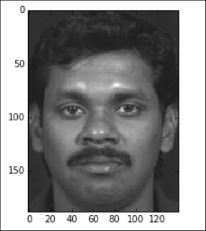
Once we have our images appropriately cleaned, how can we turn them into more general features for modeling? One approach is to try to capture common patterns of variation between a group of images using the same dimensionality reduction techniques as we used previously for document data. Instead of words in documents, we have patterns of pixels within an image, but otherwise the same algorithms and analysis largely apply. As an example, let us consider a set of images of faces (http://www.geocities.ws/senthilirtt/Senthil%20Face%20Database%20Version1) which we can load and examine using the following commands:

>>> faces = skimage.io.imread_collection('senthil_database_version1/S1/*.tif')
>>> io.imshow(faces[1])

For each of these two-dimenional images, we want to convert it into a vector just as we did when we plotted the pixel frequency histograms during our discussion of normalization. We will also construct a set where the average pixel intensity across faces has been subtracted from each pixel, yielding each face as an offset from the average face in the data through the following commands:

>>> faces_flatten = [f.ravel() for f in faces]
>>> import pylab
>>> faces_flatten_demean = pylab.demean(faces_flatten,axis=1)

We consider two possible ways to factor faces into a more general features. The first is to use PCA to extract the major vectors of variation in this data—these vectors happen to also look like faces. Since they are formed from the eigenvalues of the covariance matrix, these sorts of features are sometimes known as eigenfaces. The following commands illustrate the result of performing PCA on the face dataset:

>>> from sklearn.decomposition import PCA
>>> faces_components = PCA(n_components=3).fit(faces_flatten_demean)
>>> io.imshow(np.reshape(faces_components.components_[1],(188,140)))

How much variation in the face data is captured by the principal components? In contrast to the document data, we can see that using PCA even with only three components allows to explain around two-thirds of the variation in the dataset:

>>> plt.plot(faces_components.explained_variance_ratio_.cumsum())

We could also apply NMF, as we described previously, to find a set of basis faces. You can notice from the preceding heatmap that the eigenfaces we extracted can have negative values, which highlights one of the interpretational difficulties we mentioned previously: we cannot really have negative pixels (since , so a latent feature with negative elements is hard to interpret. In contrast, the components we extract using NMF will look much more like elements of the original dataset, as shown below using the commands:

>>> from sklearn.decomposition import NMF
>>> faces_nmf = NMF(n_components=3).fit(np.transpose(faces_flatten)) 
>>> io.imshow(np.reshape(faces_nmf.components_[0],(188,140))) 

Unlike the eigenfaces, which resemble averaged versions of many images, the NMF components extracted from this data look like individual faces. While we will not go through the exercise here, we could even apply LDA to image data to find topics represented by distributions of pixels and indeed it has been used for this purpose (Yu, Hua, and Jie Yang. A direct LDA algorithm for high-dimensional data—with application to face recognition. Pattern recognition 34.10 (2001): 2067-2070; Thomaz, Carlos E., et al. Using a maximum uncertainty LDA-based approach to classify and analyse MR brain images. Medical Image Computing and Computer-Assisted Intervention–MICCAI 2004. Springer Berlin Heidelberg, 2004. 291-300.).

While the dimensionality reduction techniques we have discussed previously are useful in the context of understanding datasets, clustering, or modeling, they are also potentially useful in storing compressed versions of data. Particularly in model services such as the one we will develop in Chapter 8, Sharing Models with Prediction Services, being able to store a smaller version of the data can reduce system load and provide an easier way to process incoming data into a form that can be understood by a predictive model. We can quickly extract the few components we need, for example, from a new piece of text data, without having to persist the entire record.