
Chapter 5
Query Processing and Execution
WHAT’S IN THIS CHAPTER?
- How SQL Server processes queries
- Understanding query optimization
- Reading query plans
- Using options to affect query plans
- Using plan hints to affect query plans
WROX.COM CODE DOWNLOADS FOR THIS CHAPTER
The wrox.com code downloads for this chapter are found at www.wrox.com/remtitle.cgi?isbn=1118177657 on the Download Code tab. The code is in the Chapter 5 download and individually named according to the names throughout the chapter.
This section uses the AdventureWorks 2012 database, so now is a good time to download it from the SQL Server section on CodePlex if you haven’t already. The AdventureWorks 2012 samples can be found at http://www.codeplex.com/SqlServerSamples.
INTRODUCTION
Query processing is one of the most critical activities that SQL Server performs in order to return data from your T-SQL queries. Understanding how SQL Server processes queries, including how they are optimized and executed, is essential to understanding what SQL Server is doing and why it chooses a particular way to do it.
In this chapter you will learn how SQL Server query processing works, including the details of query optimization and the various options that you can use to influence the optimization process; and how SQL Server schedules activities and executes them.
QUERY PROCESSING
Query processing is performed by the Relational Engine in SQL Server. It is the process of taking the T-SQL statements you write and converting them into something that can make requests to the Storage Engine and retrieve the results needed.
SQL Server takes four steps to process a query: parsing, algebrizing, optimizing, and execution. They are shown in Figure 5-1.
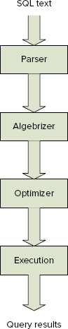
The first three steps are all performed by the Relational Engine. The output of the third step is the optimized plan that is scheduled, and during which calls are made to the Storage Engine to retrieve the data that becomes the results of the query you are executing.
Query optimization and execution are covered later in this chapter. The following sections briefly discuss parsing and algebrizing.
Parsing
During the parsing stage SQL Server performs basic checks on the source code (your T-SQL batch). This parsing looks for invalid SQL syntax, such as incorrect use of reserved words, column and table names, and so on.
If parsing completes without errors, it generates a parse tree, which is passed onto the next stage of query processing, binding. The parse tree is an internal representation of the query. If parsing detects any errors, the process stops and the errors are returned.
Algebrizing
The algebrization stage is also referred to as the binding stage. In early versions of SQL Server this stage was referred to as normalization. During algebrizing, SQL Server performs several operations on the parse tree and then generates a query tree that is passed on to the Query Optimizer.
The steps performed during algebrizing follow this model:
- Step 1: Name resolution — Confirms that all objects exist and are visible in the security context of the user. This is where the table and column names are checked to ensure that they exist and that the user has access to them.
- Step 2: Type derivation — Determines the final type for each node in the parse tree
- Step 3: Aggregate binding — Determines where to do any aggregations
- Step 4: Group binding — Binds any aggregations to the appropriate select list
Syntax errors are detected during this stage. If a syntax error is encountered, the optimization process halts and the error is returned to the user.
QUERY OPTIMIZATION
The job of the Query Optimizer is to take the query tree that was output from the algebrizer and find a “good” way to retrieve the data (results) needed. Note the use of “good” here, rather than “best,” as for any nontrivial query, there may be hundreds, or even thousands, of different ways to achieve the same results, so finding the absolutely best one can be an extremely time-consuming process. Therefore, in order to provide results in a timely manner, the Query Optimizer looks for a “good enough” plan, and uses that. This approach means that you may very well be able to do better when you manually inspect the query plan; and in the section “Influencing Optimization” you will look at different ways you can affect the decisions that SQL Server makes during optimization.
The query optimization process is based on a principle of cost, which is an abstract measure of work that is used to evaluate different query plan options. The exact nature of these costs is a closely guarded secret, with some people suggesting that they are a reflection of the time, in seconds, that the query is expected to take. They also take into account I/O and CPU resources. However, users should consider cost to be a dimensionless value that doesn’t have any units — its value is derived from comparisons to the cost of other plans in order to find the cheapest one. Therefore, there are no true units for cost values.
Although the exact details of what SQL Server does within the optimization phase are secret, it’s possible to get a glimpse at some of what goes on. For the purposes of this book, you don’t need to know every small detail, and in fact such a deep understanding isn’t useful anyway. For one thing, there is nothing you can do to alter this process; moreover, with each new service pack or hotfix, the SQL Server team tunes the internal algorithms, thereby changing the exact behavior. If you were to know too much about what was occurring, you could build in dependencies that would break with every new version of SQL Server.
Rather than know all the details, you need only understand the bigger picture. Even this bigger picture is often too much information, as it doesn’t offer any real visibility into what the Query Optimizer is doing. All you can see of this secretive process is what is exposed in the Dynamic Management View (DMV) sys.dm_exec_query_optimizer_info. This can be interesting, but it’s not a great deal of help in understanding why a given T-SQL statement is assigned a particular plan, or how you can “fix” what you think may be a non-optimal plan.
The current model provided by the SQL Server team works something like this:
- Is a valid plan cached? If yes, then use the cached plan. If no plan exists, then continue.
- Is this a trivial plan? If yes, then use the trivial plan. If no, then continue.
- Apply simplification. Simplification is a process of normalizing the query tree and applying some basic transformations to additionally “simplify” the tree.
- Is the plan cheap enough? If yes, then use this. If no, then start optimization.
- Start cost-based optimization.
- Phase 0 — Explore basic rules, and hash and nested join options.
- Does the plan have a cost of less than 0.2? If yes, then use this. If no, then continue.
- Phase 1 — Explore more rules, and alternate join ordering. If the best (cheapest) plan costs less than 1.0, then use this plan. If not, then if MAXDOP > 0 and this is an SMP system, and the min cost > cost threshold for parallelism, then use a parallel plan. Compare the cost of the parallel plan with the best serial plan, and pass the cheaper of the two to phase 2.
- Phase 2 — Explore all options, and opt for the cheapest plan after a limited number of explorations.
The output of the preceding steps is an executable plan that can be placed in the cache. This plan is then scheduled for execution, which is explored later in this chapter.
You can view the inner workings of the optimization process via the DMV sys.dm_exec_query_optimizer_info. This DMV contains a set of optimization attributes, each with an occurrence and a value. Refer to SQL Books Online (BOL) for full details. Here are a few that relate to some of the steps just described:
select *
from sys.dm_exec_query_optimizer_info
where counter in (
'optimizations'
, 'trivial plan'
, 'search 0'
, 'search 1'
, 'search 2'
)
order by [counter]
The preceding will return the same number of rows as follows, but the counters and values will be different. Note that the value for optimizations matches the sum of the trivial plan, search 0, search 1, and search 2 counters (2328 + 8559 + 3 + 17484 = 28374):
Counter               occurrencevalue
Optimizations 28374        1
search 0      2328         1
search 1      8559         1
search 2      3            1
trivial plan  17484        1
Parallel Plans
A parallel plan is any plan for which the Optimizer has chosen to split an applicable operator into multiple threads that are run in parallel.
Not all operators are suitable to be used in a parallel plan. The Optimizer will only choose a parallel plan if:
- the server has multiple processors,
- the maximum degree of parallelism setting allows parallel plans, and
- the cost threshold for parallelism sql server configuration option is set to a value lower than the lowest cost estimate for the current plan. Note that the value set here is the time in seconds estimated to run the serial plan on a specific hardware configuration chosen by the Query Optimizer team.
- The cost of the parallel plan is cheaper than the serial plan.
If all these criteria are met, then the Optimizer will choose to parallelize the operation.
An example that illustrates how this works is trying to count all the values in a table that match particular search criteria. If the set of rows in the table is large enough, the cost of the query is high enough, and the other criteria are met, then the Optimizer might parallelize the operation by dividing the total set of rows in the table into equal chunks, one for each processor core. The operation is then executed in parallel, with each processor core executing one thread, and dealing with one/number of cores of the total set of rows. This enables the operation to complete in a lot less time than using a single thread to scan the whole table. One thing to be aware of when dealing with parallel plans is that SQL Server doesn’t always do a great job of distributing the data between threads, and so your parallel plan may well end up with one or two of the parallel threads taking considerably longer to complete.
Algebrizer Trees
As mentioned earlier, the output of the parser is a parse tree. This isn’t stored anywhere permanently, so you can’t see what this looks like. The output from the algebrizer is an algebrizer tree, which isn’t stored for any T-SQL queries either, but some algebrizer output is stored — namely, views, defaults, and constraints. This is stored because these objects are frequently reused in other queries, so caching this information can be a big performance optimization. The algebrizer trees for these objects are stored in the cache store, where type = CACHESTORE_PHDR:
select *
from sys.dm_os_memory_cache_entries
where type = 'CACHESTORE_PHDR'
It’s only at the next stage (i.e., when you have the output from optimization) that things start to get really interesting, and here you can see quite a bit of information. This very useful data provides details about each optimized plan.
sql_handle or plan_handle
In the various execution-related DMVs, some contain a sql_handle, while others contain the plan_handle. Both are hashed values: sql_handle is the hash of the original T-SQL source, whereas plan_handle is the hash of the cached plan. Because the SQL queries are auto-parameterized, the relationship between these means that many sql_handles can map to a single plan_handle.
You can see the original T-SQL for either using the dynamic management function (DMF) sys.dm_exec_sql_text (sql_handle | Plan_handle).
To see the XML showplan for the plan, use the DMF sys.dm_exec_query_plan (plan_handle).
Understanding Statistics
Statistics provide critical information needed by SQL Server when performing query optimization. SQL Server statistics contain details about the data, and what the data looks like in each table within the database.
The query optimization process uses statistics to determine how many rows a query might need to access for a given query plan. It uses this information to develop its cost estimate for each step in the plan. If statistics are missing or invalid, the Query Optimizer can arrive at an incorrect cost for a step, and thus choose what ends up being a bad plan.
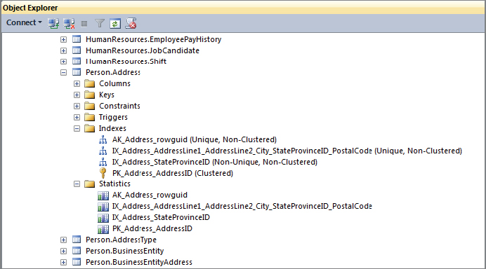
You can examine the statistics for any table in the database by using SQL Server Management Studio, expanding the Object Explorer to show the table you are interested in. For example, Figure 5-2 shows the person.Address table in the AdventureWorks2012 database. Expand the table node, under which you will see a Statistics node. Expand this, and you will see a statistic listed for each index that has been created, and in many cases you will see additional statistics listed, often with cryptic names starting with _WA. These are statistics that SQL Server has created automatically for you, based upon queries that have been run against the database. SQL Server creates these statistics when the AUTO_CREATE_STATISTICS option is set to ON.
To see the actual statistic values, you can select an individual statistic, right-click it, and select the Properties option from the menu options. This will show you the Properties dialog for the statistic you selected. The first page, General, displays the columns in the statistic and when it was last updated. The Details page contains the real guts of the statistic, and shows the data distribution. For the PK_Address-AddressID statistic on the person.Address table in AdventureWorks2012, you should see something similar to Figure 5-3.
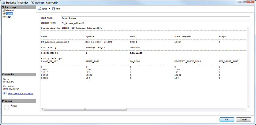
This figure shows just part of the multi-column output, which is the same output that you get when running the following DBCC command:
DBCC SHOW_STATISTICS ("Person.Address", PK_Address_AddressID);The following SQL Server configuration options control how statistics are created.
Auto_create_statistics
When this is on (default), SQL Server automatically creates statistics when it thinks they would result in a better plan. That usually means when it is optimizing a query that references a column without statistics.
Auto_update_statistics
When this is on (default), SQL Server automatically updates statistics when a sufficient amount of the data in the relevant columns has changed. By default, this is done synchronously, which means that a query has to wait for the statistics to be updated before the optimization process can be completed.
Auto_update_statistics_asynchronously
When this option is on, SQL Server updates statistics asynchronously. This means that when it’s trying to optimize a query and the statistics are outdated, it will continue optimizing the current query using the old stats, and queue the stats to be updated asynchronously. As a result, the current query doesn’t benefit from the new stats, but it does not have to wait while stats are being updated before getting a plan and running. Any future queries can then benefit from the new stats.
Plan Caching and Recompilation
Once the Query Optimizer has come up with a plan, which may have taken a considerable amount of work, SQL Server does its best to ensure that you can leverage all that costly work again. It does this by caching the plan it just created, and taking steps to ensure that the plan is reused as widely as possible. It does this by using parameterization options.
Parameterization
Parameterization is a process whereby SQL Server takes the T-SQL you entered and looks for ways to replace values that may be variables with a token, so that if a similar query is processed, SQL Server can identify it as being the same underlying query, apart from some string, or integer values, and make use of the already cached plan. For example, the following is a basic T-SQL query to return data from the AdventureWorks2012 database:
select *
from person.person
where lastname = 'duffy'
Parameterization of this query would result in the string ’duffy’ being replaced with a parameter such that if another user executes the following query, the same plan would be used, saving on compilation time:
select *
from person.person
where lastname = 'miller'
Note that this is just an example, and this particular query gets a trivial plan, so it isn’t a candidate for parameterization.
The SQL Server Books Online topic on “Forced Parameterization” contains very specific details about what can and cannot be converted to a parameter.
To determine whether a query has been parameterized, you can search for it in the DMV sys.dm_exec_cached_plans (after first executing the query to ensure it is cached). If the SQL column of this DMV shows that the query has been parameterized, any literals from the query are replaced by variables, and those variables are declared at the beginning of the batch.
Parameterization is controlled by one of two SQL Server configuration options — simple or forced:
- Simple parameterization — The default operation of SQL Server is to use simple parameterization on all queries that are suitable candidates. Books Online provides numerous details about which queries are selected and how SQL Server performs parameterization. Using simple parameterization, SQL Server is able to parameterize only a relatively small set of the queries it receives.
- Forced parameterization — For more control over database performance, you can specify that SQL Server use forced parameterization. This option forces SQL Server to parameterize all literal values in any select, insert, update, or delete statement queries. There are some exceptions to this, which are well documented in SQL Server Books Online. Forced parameterization is not appropriate in all environments and scenarios. It is recommended that you use it only for a very high volume of concurrent queries, and when you are seeing high CPU from a lot of compilation/recompilation. If you are not experiencing a lot of compilation/recompilation, then forced parameterization is probably not appropriate. Using forced in the absence of these symptoms may result in degraded performance and/or throughput because SQL Server takes more time to parameterize a lot of queries that are not later reused. It can also lead to parameter sniffing, causing inappropriate plan use.
Looking into the Plan Cache
The plan cache is built on top of the caching infrastructure provided by the SQL OS. This provides objects called cache stores, which can be used to cache all kinds of objects. The plan cache contains several different cache stores used for different types of objects.
To see the contents of a few of the cache stores most relevant to this conversation, run the following T-SQL:
select name, entries_count, pages_kb
from sys.dm_os_memory_cache_counters
where [name] in (
'object plans'
, 'sql plans'
, 'extended stored procedures'
)
Example output when I ran the preceding on my laptop is as follows:
name                       entries_count pages_kbObject Plans
54            12312SQL Plans                  48            2904Extended
Stored Procedures 4             48
Each cache store contains a hash table that is used to provide efficient storage for the many plans that may reside in the plan cache at any time. The hash used is based on the plan handle. The hash provides buckets to store plans, and many plans can reside in any one bucket. SQL Server limits both the number of plans in any bucket and the total number of hash buckets. This is done to avoid issues with long lookup times when the cache has to store a large number of plans, which can easily happen on a busy server handling many different queries.
To find performance issues caused by long lookup times, you can look into the contents of the DMV sys.dm_os_memory_cache_hash_tables, as shown in the following example. It is recommended that no bucket should contain more than 20 objects; and buckets exceeding 100 objects should be addressed.
select *
from sys.dm_os_memory_cache_hash_tables
where type in (
'cachestore_objcp'
, 'cachestore_sqlcp'
, 'cacchestore_phdr'
, 'cachestore_xproc'
)
Use the following DMV to look for heavily used buckets:
select bucketid, count(*) as entries_in_bucket
from sys.dm_exec_cached_plans
group by bucketid
order by 2 desc
You can look up the specific plans in that bucket using this query:
select *
from sys.dm_exec_cached_plans
where bucketid = 236
If the plans you find within the same bucket are all variations on the same query, then try to get better plan reuse through parameterization. If the queries are already quite different, and there is no commonality that would allow parameterization, then the solution is to rewrite the queries to be dramatically different, enabling them to be stored in emptier buckets.
Another approach is to query sys.dm_exec_query_stats, grouping on query_plan_hash to find queries with the same query plan hash using the T-SQL listed here:
select query_plan_hash,count(*) as occurrences
from sys.dm_exec_query_stats
group by query_plan_hash
having count(*) > 1
Four different kinds of objects are stored in the plan cache. Although not all of them are of equal interest, each is briefly described here:
- Algebrizer trees are the output of the algebrizer, although only the algebrizer trees for views, defaults, and constraints are cached.
- Compiled plans are the objects you will be most interested in. This is where the query plan is cached.
- Cursor execution contexts are used to track the execution state when a cursor is executing, and are similar to the next item.
- Execution contexts track the context of an individual compiled plan.
The first DMV to look at in the procedure cache is sys.dm_exec_cached_plans. The following query gathers some statistics on the type of objects exposed through this DMV (note that this doesn’t include execution contexts, which are covered next):
select cacheobjtype, objtype, COUNT (*)
from sys.dm_exec_cached_plans
group by cacheobjtype, objtype
order by cacheobjtype, objtype
Running the preceding on my laptop resulted in the following output; your results will vary according to what was loaded into your procedure cache:
CACHEOBJTYPE   OBJTYPE   (NO COLUMN NAME)
Compiled Plan  Adhoc     43
Compiled Plan  Prepared  20
Compiled Plan  Proc      54
Extended Proc  Proc      4
Parse Tree     Check     2
Parse Tree     UsrTab    1
Parse Tree     View      64
To see the execution contexts, you must pass a specific plan handle to sys.dm_exec_cached_plans_dependent_objects. However, before doing that, you need to find a plan_handle to pass to this dynamic management function (DMF). To do that, run the following T-SQL:
-- Run this to empty the cache
-- WARNING !!! DO NOT TRY THIS ON A PRODUCTION SYSTEM !!!
dbcc freeproccache
Now see how many objects there are in the cache. There will always be a bunch of stuff here from the background activities that SQL is always running.
select cacheobjtype, objtype, COUNT (*)
from sys.dm_exec_cached_plans
group by cacheobjtype, objtype
order by cacheobjtype, objtype
The output of the query will look similar to this:
CACHEOBJTYPE    OBJTYPE    (NO COLUMN NAME)
Compiled Plan   Adhoc      5
Compiled Plan   Prepared   1
Compiled Plan   Proc       11
Extended Proc   Proc       1
Parse Tree      View       10
Run the following code in the AdventureWorks2012 database, from another connection:
select lastname, COUNT (*)
from Person.Person_test
group by lastname
order by 2 desc
The output of the prior query is not of interest, so it’s not shown here. The following query goes back and reexamines the cache:
-- Check that we got additional objects into the cache
select cacheobjtype, objtype, COUNT (*)
from sys.dm_exec_cached_plans
group by cacheobjtype, objtype
order by cacheobjtype, objtype
The output of the query will look similar to this:
CACHEOBJTYPE    OBJTYPE    (NO COLUMN NAME)
Compiled Plan   Adhoc      9
Compiled Plan   Prepared   2
Compiled Plan   Proc       14
Extended Proc   Proc       2
Parse Tree      View       13
At this point you can see that there are four more ad hoc compiled plans, and a number of other new cached objects. The objects you are interested in here are the ad hoc plans.
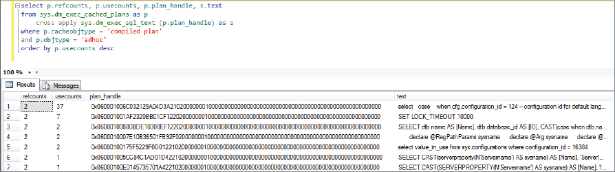
Run the following T-SQL to get the SQL text and the plan handle for the T-SQL query you ran against the AdventureWorks2012 database:
select p.refcounts, p.usecounts, p.plan_handle, s.text
from sys.dm_exec_cached_plans as p
    cross apply sys.dm_exec_sql_text (p.plan_handle) as s
where p.cacheobjtype = 'compiled plan'
and p.objtype = 'adhoc'
order by p.usecounts desc
This should provide something similar to the results shown in Figure 5-4.
To see the execution context, take the plan_handle that you got from the preceding results and plug it into the DMF sys.dm_exec_cached_plan_dependent_objects, as shown in the following example:
select *
from sys.dm_exec_cached_plan_dependent_objects
(0x06000F005163130CB880EE0D000000000000000000000000)
The preceding code returned the following results:
USECOUNTS MEMORY_OBJECT_ADDRESS CACHEOBJTYPE
1         0x0DF8A038            Executable Plan
Another interesting thing you can examine are the attributes of the plan. These are found in the DMF sys.dm_exec_plan_attributes (plan_handle) Note that you need to pass the DMF a plan handle, and then you will get the attributes for that plan:
select *
from sys.dm_exec_plan_attributes
(0x06000F00C080471DB8E06914000000000000000000000000)
The preceding query outputs a list of 28 attributes, a select few of which are shown here:
ATTRIBUTE       VALUE                                              IS_CACHE_KEY
set_options     135419                                             1
objectid        491225280                                          1
dbid            15                                                 1
language_id     0                                                  1
date_format     1                                                  1
date_first      7                                                  1
compat_level    100                                                1
sql_handle      0x02000000C080471DB475BDA81DA97B1C6F2EEA51417711E8 0
The sql_handle in these results can then be used in a call to the DMF sys.dm_exec_sql_text (sql_handle) to see the SQL that was being run.
Compilation/Recompilation
Compilation and recompilation are pretty much the same thing, just triggered at slightly different times. When SQL Server decides that an existing plan is no longer valid, which is usually due to a schema change, statistics changes, or some other event, it will re-compile the plan. This happens only when someone tries to run the query. If they try to run the query when no one else is using the plan, it is a compile event. If this happens when someone else is using a copy of the plan, it is a recompile event.
You can monitor the amount of compilation/recompilation that’s occurring by observing the PerfMon Object SQL Server: SQL Statistics and then looking at the following two counters: SQL compilations/sec and SQL recompilations/sec.
Influencing Optimization
There are two main ways you can influence the Query Optimizer — by using query hints or plan guides.
Query Hints
Query hints are an easy way to influence the actions of query optimization. However, you need to very carefully consider their use, as in most cases SQL Server is already choosing the right plan. As a general rule, you should avoid using query hints, as they provide many opportunities to cause more issues than the one you are attempting to solve. In some cases, however, such as with complex queries or when dealing with complex datasets that defeat SQL Server’s cardinality estimates on specific queries, using query hints may be necessary.
Before using any query hints, run a web search for the latest information on issues with query hints. Try searching on the keywords “SQL Server Query Hints” and look specifically for anything by Craig Freedman, who has written several great blog entries on some of the issues you can encounter when using query hints.
Problems with using hints can happen at any time — from when you start using the hint, which can cause unexpected side effects that cause the query to fail to compile, to more complex and difficult to find performance issues that occur later.
As data in the relevant tables changes, without query hints the Query Optimizer automatically updates statistics and adjusts query plans as needed; but if you have locked the Query Optimizer into a specific set of optimizations using query hints, then the plan cannot be changed, and you may end up with a considerably worse plan, requiring further action (from you) to identify and resolve the root cause of the new performance issue.
One final word of caution about using query hints: Unlike locking hints (also referred to in BOL as table hints), which SQL Server attempts to satisfy, query hints are stronger, so if SQL Server is unable to satisfy a query hint it will raise error 8622 and not create any plan.
Query hints are specified using the OPTION clause, which is always added at the end of the T-SQL statement — unlike locking or join hints, which are added within the T-SQL statement after the tables they are to affect.
The following sections describe a few of the more interesting query hints.
FAST number_rows
Use this query hint when you want to retrieve only the first n rows out of a relatively large result set. A typical example of this is a website that uses paging to display large sets of rows, whereby the first page shows only the first web page worth of rows, and a page might contain only 20, 30, or maybe 40 rows. If the query returns thousands of rows, then SQL Server would possibly optimize this query using hash joins. Hash joins work well with large datasets but have a higher setup time than perhaps a nested loop join. Nested loop joins have a very low setup cost and can return the first set of rows more quickly but takes considerably longer to return all the rows. Using the FAST <number_rows> query hint causes the Query Optimizer to use nested loop joins and other techniques, rather than hashed joins, to get the first n rows faster.
Typically, once the first n rows are returned, if the remaining rows are retrieved, the query performs slower than if this hint were not used.
{Loop | Merge | Hash } JOIN
The JOIN query hint applies to all joins within the query. While this is similar to the join hint that can be specified for an individual join between a pair of tables within a large more complex query, the query hint applies to all joins within the query, whereas the join hint applies only to the pair of tables in the join with which it is associated.
To see how this works, here is an example query using the AdventureWorks2012 database that joins three tables. The first example shows the basic query with no join hints.
use AdventureWorks2012
go

set statistics profile on
go

select p.title, p.firstname, p.middlename, p.lastname
, a.addressline1, a.addressline2, a.city, a.postalcode
from person.person as p inner join person.businessentityaddress as b
on p.businessentityid = b.businessentityid
inner join person.address as a on b.addressid = a.addressid
go

set statistics profile off
go
This returns two result sets. The first is the output from the query, and returns 18,798 rows; the second result set is the additional output after enabling the set statistics profile option. One interesting piece of information in the statistics profile output is the totalsubtreecost column. To see the cost for the entire query, look at the top row. On my test machine, this query is costed at 4.649578. The following shows just the PhysicalOp column from the statistics profile output, which displays the operator used for each step of the plan:
PHYSICALOP
NULL
Merge Join
Clustered Index Scan
Sort
Merge Join
Clustered Index Scan
Index Scan
The next example shows the same query but illustrates the use of a table hint. In this example the join hint applies only to the join between person.person and person.businessentity:
use AdventureWorks2012
go

set statistics profile on
go

select p.title, p.firstname, p.middlename, p.lastname
, a.addressline1, a.addressline2, a.city, a.postalcode
from person.person as p inner loop join person.businessentityaddress as b
on p.businessentityid = b.businessentityid
inner join person.address as a on b.addressid = a.addressid
go

set statistics profile off
go
The totalsubtree cost for this option is 8.155532, which is quite a bit higher than the plan that SQL chose, and indicates that our meddling with the optimization process has had a negative impact on performance.
The PhysicalOp column of the statistics profile output is shown next. This indicates that the entire order of the query has been dramatically changed; the merge joins have been replaced with a loop join as requested, but this forced the Query Optimizer to use a hash match join for the other join. You can also see that the Optimizer chose to use a parallel plan, and even this has not reduced the cost:
PhysicalOp
NULL
Parallelism
Hash Match
Parallelism
Nested Loops
Clustered Index Scan
Clustered Index Seek
Parallelism
Index Scan
The final example shows the use of a JOIN query hint. Using this forces both joins within the query to use the join type specified:
use AdventureWorks2012
go

set statistics profile on
go

select p.title, p.firstname, p.middlename, p.lastname
, a.addressline1, a.addressline2, a.city, a.postalcode
from person.person as p inner join person.businessentityaddress as b
on p.businessentityid = b.businessentityid
inner join person.address as a on b.addressid = a.addressid
option (hash join )
go

set statistics profile off
go
The total subtreecost for this plan is 5.097726. This is better than the previous option but still worse than the plan chosen by SQL Server.
The PhysicalOp column of the following statistics profile output indicates that both joins are now hash joins:
PhysicalOp
NULL
Parallelism
Hash Match
Parallelism
Hash Match
Parallelism
Index Scan
Parallelism
Clustered Index Scan
Parallelism
Index Scan
Using a query hint can cause both compile-time and runtime issues. The compile-time issues are likely to happen when SQL Server is unable to create a plan due to the query hint. Runtime issues are likely to occur when the data has changed enough that the Query Optimizer needs to create a new plan using a different join strategy but it is locked into using the joins defined in the query hint.
MAXDOP n
The MAXDOP query hint is only applicable on systems and SQL Server editions for which parallel plans are possible. On single-core systems, multiprocessor systems where CPU affinity has been set to a single processor core, or systems that don’t support parallel plans (i.e. if you are running the express edition of SQL Server which can only utilize a single processor core), this query hint has no effect.
On systems where parallel plans are possible, and in the case of a query where a parallel plan is being generated, using MAXDOP (n) allows the Query Optimizer to use only n workers.
On very large SMPs or NUMA systems, where the SQL Server configuration setting for Max Degree of Parallelism is set to a number less than the total available CPUs, this option can be useful if you want to override the systemwide Max Degree of Parallelism setting for a specific query.
A good example of this might be a 16 core SMP server with an application database that needs to service a large number of concurrent users, all running potentially parallel plans. To minimize the impact of any one query, the SQL Server configuration setting Max Degree of Parallelism is set to 4, but some activities have a higher “priority” and you want to allow them to use all CPUs. An example of this might be an operational activity such as an index rebuild, when you don’t want to use an online operation and you want the index to be created as quickly as possible. In this case, the specific queries for index creation/rebuilding can use the MAXDOP 16 query hint, which allows SQL Server to create a plan that uses all 16 cores.
OPTIMIZE FOR
Because of the extensive use of plan parameterization, and the way that the Query Optimizer sniffs for parameters on each execution of a parameterized plan, SQL Server doesn’t always do the best job of choosing the right plan for a specific set of parameters.
The OPTIMIZE FOR hint enables you to tell the Query Optimizer what values you expect to see most commonly at runtime. Provided that the values you specify are the most common case, this can result in better performance for the majority of the queries, or at least those that match the case for which you optimized.
RECOMPILE
The RECOMPILE query hint is a more granular way to force recompilation in a stored procedure to be at the statement level rather than using the WITH RECOMPILE option, which forces the whole stored procedure to be recompiled.
When the Query Optimizer sees the RECOMPILE query hint, it forces a new query plan to be created regardless of what plans may already be cached. The new plan is created with the parameters within the current execution context.
This is a very useful option if you know that a particular part of a stored procedure has very different input parameters that can affect the resulting query plan dramatically. Using this option may incur a small cost for the compilation needed on every execution, but if that’s a small percentage of the resulting query’s execution time, it’s a worthwhile cost to pay to ensure that every execution of the query gets the most optimal plan.
For cases in which the additional compilation cost is high relative to the cost of the worst execution, using this query hint would be detrimental to performance.
USE PLAN N ‘xml plan’
The USE PLAN query hint tells the Query Optimizer that you want a new plan, and that the new plan should match the shape of the plan in the supplied XML plan.
This is very similar to the use of plan guides (covered in the next section), but whereas plan guides don’t require a change to the query, the USE PLAN query hint does require a change to the T-SQL being submitted to the server.
Sometimes this query hint is used to solve deadlock issues or other data-related problems. However, in nearly all cases the correct course of action is to address the underlying issue, but that often involves architectural changes, or code changes that require extensive development and test work to get into production. In these cases the USE PLAN query hint can provide a quick workaround for the DBA to keep the system running while the root cause of a problem is found and fixed.
Note that the preceding course of action assumes you have a “good” XML plan from the problem query that doesn’t show the problem behavior. If you just happened to capture a bunch of XML plans from all the queries running on your system when it was working well, then you are good to go, but that’s not typically something that anyone ever does, as you usually leave systems alone when they are working OK; and capturing XML plans for every query running today just in case you may want to use the USE PLAN query hint at some point in the future is not a very useful practice.
What you may be able to do, however, is configure a test system with data such that the plan your target query generates is of the desired shape, capture the XML for the plan, and use that XML plan to “fix” the plan’s shape on your production server.
Plan Guides
Plan guides, which were added in SQL Server 2005, enable the DBA to affect the optimization of a query without altering the query itself. Typically, plan guides are used by DBAs seeking to tune query execution on third-party application databases, where the T-SQL code being executed is proprietary and cannot be changed. Typical examples of applications for which plan guides are most likely to be needed would be large ERP applications such as SAP, PeopleSoft, and so on.
Although plan guides were first added in SQL Server 2005, significant enhancements, primarily regarding ease of use, were made to them in SQL Server 2008.
There are three different types of plan guide:
- Object plan guide — Can be applied to a stored procedure, trigger, or user-defined function
- SQL plan guide — Applied to a specific SQL statement
- Template plan guide — Provides a way to override database settings for parameterization of specific SQL queries
To make use of plan guides, the first step is to create or capture a “good” plan; the second step is to apply that plan to the object or T-SQL statement for which you want to change the Query Optimizer’s behavior.
QUERY PLANS
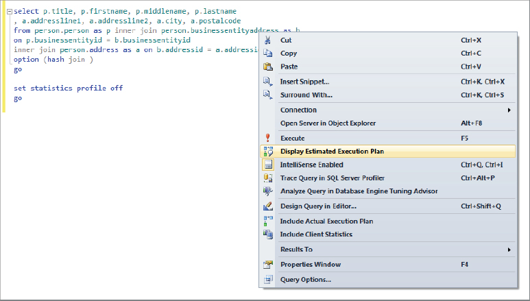
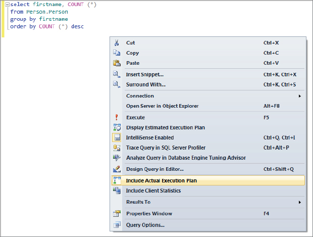
Now that you have seen how your T-SQL is optimized, the next step is to look at the query plan that the Query Optimizer generated for it. There are several ways to view query plans, but perhaps the easiest is to view the graphical plan using SQL Server Management Studio (SSMS). SSMS makes this extra easy by providing a context-sensitive menu option that enables you to highlight any piece of T-SQL in a query window and display the estimated execution plan, as shown in Figure 5-5.
This provided the output shown in Figure 5-6.
You can also include SET statements with your query to enable several options that provide additional output displaying the query plan for you. These options are SHOWPLAN_TEXT and SHOWPLAN_ALL. The following code example demonstrates how to use these options:
Use AdventureWorks2012
go
set showplan_text on
go
select * from person.person
go
set showplan_text off
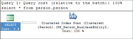
goFollowing are the two result sets returned by this query. Note that this is the output after setting the query result options to results to text, rather than results to grid:
StmtText

select * from person.person

(1 row(s) affected)

StmtText
  |--Clustered Index Scan(OBJECT:([AdventureWorks2012].[Person].[Person]
.[PK_Person_BusinessEntityID]))

(1 row(s) affected)
Use AdventureWorks2012
go
set showplan_all on
go
select * from person.person
go
set showplan_all off
go
Some of the output columns from this query are shown in Figure 5-7.
You can also use SHOWPLAN_XML to get the plan in an XML format:
Use AdventureWorks2012
go
set showplan_xml on
go
select * from person.person
go
set showplan_xml off
go
The results from the preceding query are shown in Figure 5-8.
Clicking on the XML will display the graphical execution plan shown in Figure 5-9.
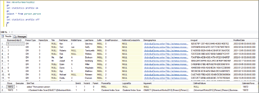
Another option is STATISTICS PROFILE. This is the first option to be discussed that executes the query, and returns a real plan. The previous options don’t execute the query, they just return an estimated plan. Enabling this option adds statistical information to the showplan. This consists of the actual row count and the number of times each operator was run when the query was executed:
Use AdventureWorks2012
go
set statistics profile on
go
select * from person.person
go
set statistics profile off
go
Some of the columns’ output from this query is shown in Figure 5-10.
Another place to look for query plans is in the plan cache itself. When dealing with a lot of queries on a busy production system, it’s often necessary to find the query plan for a particular query that’s currently being used. To do this, use the following T-SQL to return either the XML for the plan or the text of the plan:
Select *
From sys.dm_exec_query_plan(plan_handle)

Select *
From sys.dm_exec_text_query_plan(plan_handle)
Note that you can use two DMFs here: One refers to returning the XML plan; whereas the name of the other implies it will return the text of the plan, suggesting it would be similar to the showplan_text output; but, in fact, both return the XML format of the plan. The difference is that the data type of the query_plan column in one is XML, whereas the data type in the other result set is text.
Query Plan Operators
The Query Optimizer can use many different operators to create your plan. Covering them all is beyond the scope of this book, so this section instead focuses on some examples demonstrating the most common operators you will come across. For a full list of operators, refer to SQL Server Books Online (SQL BOL). Search for the topic “Showplan Logical and Physical Operators Reference.”
Join Operators
Join operators enable SQL Server to find matching rows between two tables. Prior to SQL Server 2005, there was only a single join type, the nested loop join, but since then additional join types have been added, and SQL Server now provides the three join types described in Table 5-1. These join types handle rows from two tables; for a self-join, the inputs may be different sets of rows from the same table.
TABLE 5-1: SQL Server Join Types
| JOIN TYPE | BENEFIT |
| Nested loop | Good for small tables where there is an index on the inner table on the join key |
| Merge join | Good for medium-size tables where there are ordered indexes, or where the output needs to be ordered |
| Hash join | Good for medium to large tables. Works well with parallel plans, and scales well. |
Nested Loop
The nested loop join is the original SQL Server join type. The behavior of a nested loop is to scan all the rows in one table (the outer table) and for each row in that table, it then scans every row in the other table (the inner table). If the rows in the outer and inner tables match, then the row is included in the results.
The performance of this join is directly proportional to the number of rows in each table. It performs well when there are relatively few rows in one of the tables, which would be chosen as the inner table, and more rows in the other table, which would be used as the outer table. If both tables have a relatively large number of rows, then this join starts to take a very long time.
Merge
The merge join needs its inputs to be sorted, so ideally the tables should be indexed on the join column. Then the operator iterates through rows from both tables at the same time, working down the rows, looking for matches. Because the inputs are ordered, this enables the join to proceed quickly, and to end as soon as any range is satisfied.
Hash
The hash join operates in two phases. During the first phase, known as the build phase, the smaller of the two tables is scanned and the rows are placed into a hash table that is ideally stored in memory; but for very large tables, it can be written to disk. When every row in the build input table is hashed, the second phase starts. During the second phase, known as the probe phase, rows from the larger of the two tables are compared to the contents of the hash table, using the same hashing algorithm that was used to create the build table hash. Any matching rows are passed to the output.
The hash join has variations on this processing that can deal with very large tables, so the hash join is the join of choice for very large input tables, especially when running on multiprocessor systems where parallel plans are allowed.
- Increase memory on the server.
- Make sure statistics exist on the join columns.
- Make sure statistics are current.
- Force a different type of join.
Spool Operators
The various spool operators are used to create a temporary copy of rows from the input stream and deliver them to the output stream. Spools typically sit between two other operators: The one on the right is the child, and provides the input stream. The operator on the left is the parent, and consumes the output stream.
The following list provides a brief description of each of the physical spool operators. These are the operators that actually execute. You may also see references to logical operators, which represent an earlier stage in the optimization process; these are subsequently converted to physical operators before executing the plan. The logical spool operators are Eager Spool, and Lazy Spool.
- Index spool — This operator reads rows from the child table, places them in tempdb, and creates a nonclustered index on them before continuing. This enables the parent to take advantage of seeking against the nonclustered index on the data in tempdb when the underlying table has no applicable indexes.
- Row count spool — This operator reads rows from the child table and counts the rows. The rows are also returned to the parent, but without any data. This enables the parent to determine whether rows exist in order to satisfy an EXISTS or NOT EXISTS requirement.
- Table spool — This operator reads the rows from the child table and writes them into tempdb. All rows from the child are read and placed in tempdb before the parent can start processing rows.
- Window spool — This operator expands each row into the set of rows that represent the window associated with it. It’s both a physical and logical operator.
Scan and Seek Operators
These operators enable SQL Server to retrieve rows from tables and indexes when a larger number of rows is required. This behavior contrasts with the individual row access operators key lookup and RID lookup, which are discussed in the next section.
- Scan operator — The scan operator scans all the rows in the table looking for matching rows. When the number of matching rows is >20 percent of the table, scan can start to outperform seek due to the additional cost of traversing the index to reach each row for the seek.
- Seek operator — The seek operator uses the index to find matching rows; this can be either a single value, a small set of values, or a range of values. When the query needs only a relatively small set of rows, seek is significantly faster than scan to find matching rows. However, when the number of rows returned exceeds 20 percent of the table, the cost of seek will approach that of scan; and when nearly the whole table is required, scan will perform better than seek.
Lookup Operators
Lookup operators perform the task of finding a single row of data. The following is a list of common operators:
- Bookmark lookup — Bookmark lookup is seen only in SQL Server 2000 and earlier. It’s the way that SQL Server looks up a row using a clustered index. In SQL Server 2012 this is done using either Clustered Index Seek, RID lookup, or Key Lookup.
- Key lookup — Key lookup is how a single row is returned when the table has a clustered index. In contrast with dealing with a heap, the lookup is done using the clustering key. The key lookup operator was added in SQL Server 2005 SP2. Prior to this, and currently when viewing the plan in text or XML format, the operator is shown as a clustered index seek with the keyword lookup.
- RID lookup — RID lookup is how a single row is looked up in a heap. RID refers to the internal unique row identifier (hence RID), which is used to look up the row.
Reading Query Plans
Unlike reading a typical book such as this one, whereby reading is done from top left to bottom right (unless you’re reading a translation for which the language is read in reverse), query plans in all forms are read bottom right to top left.
Once you have downloaded and installed the sample database, to make the examples more interesting you need to remove some of the indexes that the authors of AdventureWorks added for you. To do this, you can use either your favorite T-SQL scripting tool or the SSMS scripting features, or run the AW2012_person_drop_indexes.sql sample script (available on the book’s website in the Chapter 5 Samples folder, which also contains a script to recreate the indexes if you want to return the AdventureWorks2012 database to its original structure). This script drops all the indexes on the person.person table except for the primary key constraint.
After you have done this, you can follow along with the examples, and you should see the same results.
You will begin by looking at some trivial query plans, starting with a view of the graphical plans but quickly switching to using the text plan features, as these are easier to compare against one another, especially when you start looking at larger plans from more complex queries.
Here is the first trivial query to examine:
select firstname, COUNT (*)
from Person.Person
group by firstname
order by COUNT (*) desc
After running this in SSMS after enabling the Include Actual Execution Plan option, which is shown in Figure 5-11, three tabs are displayed. The first is Results, but the one you are interested in now is the third tab, which shows the graphical execution plan for this query.
You should see something like the image shown in Figure 5-12.
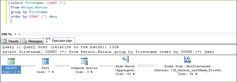
Starting at the bottom right, you can see that the first operator is the clustered index scan operator. While the query doesn’t need, or get any benefit from, a clustered index, because the table has a clustered index and is not a heap, this is the option that SQL Server chooses to read through all the rows in the table. If you had removed the clustered index, so that this table was a heap, then this operator would be replaced by a table scan operator. The action performed by both operators in this case is identical, which is to read every row from the table and deliver them to the next operator.
The next operator is the hash match. In this case, SQL Server is using this to sort the rows into buckets by first name. After the hash match is the compute scalar, whereby SQL Server counts the number of rows in each hash bucket, which gives you the count (*) value in the results. This is followed by the sort operator, which is there to provide the ordered output needed from the T-SQL.
You can find additional information on each operation by hovering over the operator. Figure 5-13 shows the additional information available on the non-clustered index scan operator.

While this query seems pretty trivial, and you may have assumed it would generate a trivial plan because of the grouping and ordering, this is not a trivial plan. You can tell this by monitoring the results of the following query before and after running it:
select *
from sys.dm_exec_query_optimizer_info
where counter in (
'optimizations'
, 'trivial plan'
, 'search 0'
, 'search 1'
, 'search 2'
)
order by [counter]
Once the query has been optimized and cached, subsequent runs will not generate any updates to the Query Optimizer stats unless you flush the procedure cache using dbcc freeproccache.
On the machine I am using, the following results were returned from this query against the Query Optimizer information before I ran the sample query:
COUNTER         OCCURRENCE  VALUE
optimizations   10059       1
search 0        1017        1
search 1        3385        1
search 2        1           1
trivial plan    5656        1
Here are the results after I ran the sample query:
COUNTER         OCCURRENCE  VALUE
optimizations   10061       1
search 0        1017        1
search 1        3387        1
search 2        1           1
trivial plan    5656        1
From this you can see that the trivial plan count didn’t increment, but the search 1 count did increment, indicating that this query needed to move onto phase 1 of the optimization process before an acceptable plan was found.
If you want to play around with this query to see what a truly trivial plan would be, try running the following:
select lastname
from person.person
The following T-SQL demonstrates what the same plan looks like in text mode:
set statistics profile on
go

select firstname, COUNT (*)
from Person.Person
group by firstname
order by 2 desc
go

set statistics profile off
go
When you run this batch, rather than see a third tab displayed in SSMS, you will see that there are now two result sets in the query’s Results tab. The first is the output from running the query, and the second is the text output for this plan, which looks something like what is shown in Figure 5-14.
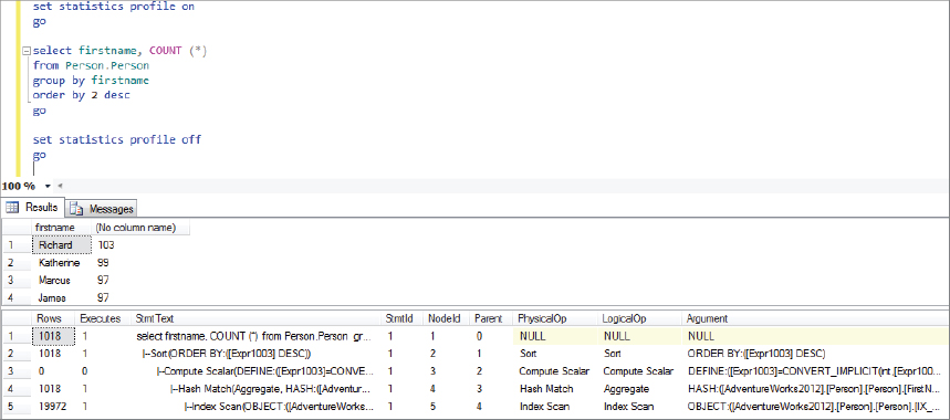
The following example shows some of the content of the StmtText column, which illustrates what the query plan looks like, just as in the graphical plan but this time in a textual format:
  |--Sort(ORDER BY:([Expr1003] DESC))
       |--Compute Scalar(DEFINE:([Expr1003 ...
            |--Hash Match(Aggregate, ...
|--Index Scan(OBJECT:( ...As mentioned before, this is read from the bottom up. You can see that the first operator is the clustered index scan, which is the same operator shown in Figure 5-6. From there (working up), the next operator is the hash match, followed by the compute scalar operator, and then the sort operator.
While the query you examined may seem pretty simple, you have noticed that even for this query, the Query Optimizer has quite a bit of work to do. As a follow-up exercise, try adding one index at a time back into the Person table, and examine the plan you get each time a new index is added. One hint as to what you will see is to add the index IX_Person_Lastname_firstname_middlename first.
From there you can start to explore with simple table joins, and look into when SQL Server chooses each of the three join operators it offers: nested loop, merge, and hash joins.
EXECUTING YOUR QUERIES
So far in this chapter, you have learned how SQL Server parses, algebrizes, and optimizes the T-SQL you want to run. This section describes how SQL Server executes the query plan. First, however, it is useful to step back a little and look at the larger picture — namely, how the SQL Server architecture changed with SQL Server 2005 and the introduction of SQLOS.
SQLOS
SQL Server 2005 underwent a major change in the underlying architecture with the introduction of SQLOS. This component provides basic services to the other SQL Server components, such as the Relational Engine and the Storage Engine. This architecture is illustrated in the diagram shown in Figure 5-15.
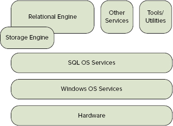
The main services provided by SQLOS are scheduling, which is where our main interest lies; and memory management, which we also have an interest in because the memory management services are where the procedure cache lives, and that’s where your query plans live. SQLOS also provides many more services that are not relevant to the current discussion. For more details on the other services provided by SQLOS, refer to Chapter 1 or SQL Server Books Online.
SQLOS implements a hierarchy of system objects that provide the framework for scheduling. Figure 5-16 shows the basic hierarchy of these objects — from the parent node, SQLOS, down to the workers, tasks, and OS threads where the work is actually performed.

The starting point for scheduling and memory allocation is the memory node.
Memory Nodes
The SQLOS memory node is a logical container for memory associated with a node, which is a collection of CPUs with shared memory. This can be either a “real” memory node, if the server has a NUMA architecture, or an artificial grouping that you created as a “soft” NUMA configuration. You’ll find more details on NUMA in Chapter 3.
Along with the memory nodes created to model the physical hardware of the server, there is always one additional memory node used by the dedicated administrator connection (DAC). This ensures that some resources are always available to service the DAC, even when all other system resources are being used.
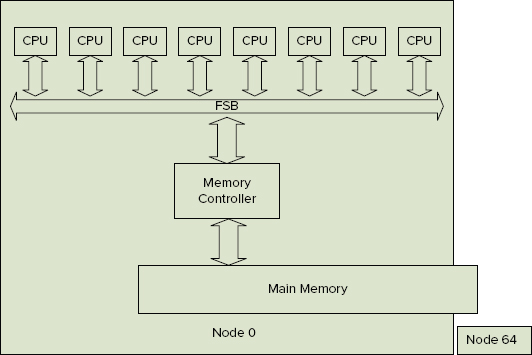
On an eight-processor SMP system without soft NUMA, there is one memory node for general server use, and one for the DAC. This is illustrated in Figure 5-17.
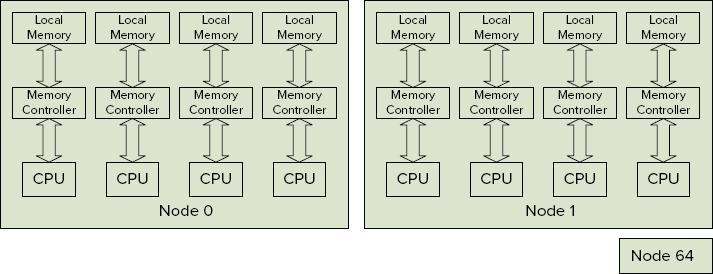
On an eight-processor NUMA system with two nodes of four cores, there would be two memory nodes for general use, and a third for the DAC. This is illustrated in Figure 5-18.
By querying the DMV sys.dm_os_memory_nodes, you can view the layout of memory nodes on your server. However, it makes more sense to include the node_state_desc column from sys.dm_os_nodes using this query. Note the join between node_id in sys.dm_os_nodes and memory_node_id in sys.dm_os_memory_nodes:
select c.node_id, c.memory_node_id, m.memory_node_id, c.node_state_desc
, c.cpu_affinity_mask, m.virtual_address_space_reserved_kb
from sys.dm_os_nodes as c inner join sys.dm_os_memory_nodes as m
on c.node_id = m.memory_node_id
Here is the output from the preceding query when run on a 16-way SMP server:
NODE_ID MEMORY_NODE_ID MEMORY_NODE_ID NODE_STATE_DESC CPU_AFFINITY_MASK VIRTUAL_ADDRESS_SPACE_RESERVED_KB
0       0               0               ONLINE           65535             67544440
64      0               64              ONLINE DAC      0                 2560
In this case, Node 0 has nearly all the 64GB of memory on this server reserved, and Node 64 is reserved for the DAC, which has just 2.5MB of memory reserved.
Following is the output from this query on a 192-processor NUMA system. The server is structured as eight NUMA nodes. Each NUMA node has four sockets, and each socket has six cores (using Intel Xeon hexa-core processors), resulting in 24 cores per NUMA node:
NODE_ID MEMORY_NODE_ID MEMORY_NODE_ID NODE_STATE_DESC CPU_AFFINITY_MASK    VIRTUAL_ADDRESS_SPACE_RESERVED_KB
0       0               0               ONLINE           16777215             268416
1       1               1               ONLINE           16777215             248827056
2       2               2               ONLINE           16777215             22464
3       3               3               ONLINE           16777215             8256
4       4               4               ONLINE           281474959933440      11136
5       5               5               ONLINE           281474959933440      4672
6       6               6               ONLINE           281474959933440      4672
7       7               7               ONLINE           281474959933440      5120
64      0               64              ONLINE DAC      0                    2864
Soft NUMA
In some scenarios, you may be able to work with an SMP server and still get the benefit of having a NUMA-type structure with SQL Server. You can achieve this by using soft NUMA. This enables you to use Registry settings to tell SQL Server that it should configure itself as a NUMA system, using the CPU-to-memory-node mapping that you specify.
As with anything that requires Registry changes, you need to take exceptional care, and be sure you have backup and rollback options at every step of the process.
One common use for soft NUMA is when a SQL Server is hosting an application that has several different groups of users with very different query requirements. After configuring your theoretical 16-processor server for soft NUMA, assigning 2 NUMA nodes with 4 CPUs , and one 8-CPU node to a third NUMA node, you would next configure connection affinity for the three nodes to different ports, and then change the connection settings for each class of workload, so that workload A is “affinitized” to port x, which connects to the first NUMA node; workload B is affinitized to port y, which connects to the second NUMA node; and all other workloads are affinitized to port z, which is set to connect to the third NUMA node.
CPU Nodes
A CPU node is a logical collection of CPUs that share some common resource, such as a cache or memory. CPU nodes live below memory nodes in the SQLOS object hierarchy.
Whereas a memory node may have one or more CPU nodes associated with it, a CPU node can be associated with only a single memory node. However, in practice, nearly all configurations have a 1:1 relationship between memory nodes and CPU nodes.
CPU nodes can be seen in the DMV sys.dm_os_nodes. Use the following query to return select columns from this DMV:
select node_id, node_state_desc, memory_node_id, cpu_affinity_mask
from sys.dm_os_nodes
The results from this query, when run on a single-CPU system are as follows:
NODE_ID NODE_STATE_DESC MEMORY_NODE_ID CPU_AFFINITY_MASK
0       ONLINE          0              1
32      ONLINE DAC      0              0
The results from the previous query, when run on a 96-processor NUMA system, comprising four nodes of four sockets, each socket with six cores, totaling 24 cores per NUMA node, and 96 cores across the whole server, are as follows:
NODE_ID NODE_STATE_DESC MEMORY_NODE_ID CPU_AFFINITY_MASK
0       ONLINE          1              16777215
1       ONLINE          0              281474959933440
2       ONLINE          2              16777215
3       ONLINE          3              281474959933440
64 ONLINE DAC 0 1677721516777215 = 0x00FFFFFF
281474959933440 = 0x0F000001000000FFFFFF0000Processor Affinity
CPU affinity is a way to force a workload to use specific CPUs. It’s another way that you can affect scheduling and SQL Server SQLOS configuration.
CPU affinity can be managed at several levels. Outside SQL Server, you can use the operating system’s CPU affinity settings to restrict the CPUs that SQL Server as a process can use. Within SQL Server’s configuration settings, you can specify that SQL Server should use only certain CPUs. This is done using the affinity mask and affinity64 mask configuration options. Changes to these two options are applied dynamically, which means that schedulers on CPUs that are either enabled or disabled while SQL is running will be affected immediately. Schedulers associated with CPUs that are disabled will be drained and set to offline. Schedulers associated with CPUs that are enabled will be set to online, and will be available for scheduling workers and executing new tasks.
You can also set SQL Server I/O affinity using the affinity I/O mask option. This option enables you to force any I/O-related activities to run only on a specified set of CPUs. Using connection affinity as described earlier in the section “Soft NUMA,” you can affinitize network connections to a specific memory node.
Schedulers
The scheduler node is where the work of scheduling activity occurs. Scheduling occurs against tasks, which are the requests to do some work handled by the scheduler. One task may be the optimized query plan that represents the T-SQL you want to execute; or, in the case of a batch with multiple T-SQL statements, the task would represent a single optimized query from within the larger batch.
When SQL Server starts up, it creates one scheduler for each CPU that it finds on the server, and some additional schedulers to run other system tasks. If processor affinity is set such that some CPUs are not enabled for this instance, then the schedulers associated with those CPUs will be set to a disabled state. This enables SQL Server to support dynamic affinity settings.
While there is one scheduler per CPU, schedulers are not bound to a specific CPU, except in the case where CPU affinity has been set.
Each scheduler is identified by its own unique scheduler_id. Values from 0–254 are reserved for schedulers running user requests. Scheduler_id 255 is reserved for the scheduler for the dedicated administrator connection (DAC). Schedulers with a scheduler_id > 255 are reserved for system use and are typically assigned the same task.
The following code sample shows select columns from the DMV sys.dm_os_schedulers:
select parent_node_id, scheduler_id, cpu_id, status, scheduler_address
from sys.dm_os_schedulers
order by scheduler_id
The following results from the preceding query indicate that scheduler_id 0 is the only scheduler with an id < 255, which implies that these results came from a single-core machine. You can also see a scheduler with an ID of 255, which has a status of VISIBLE ONLINE (DAC), indicating that this is the scheduler for the DAC. Also shown are three additional schedulers with IDs > 255. These are the schedulers reserved for system use.
PARENT_NODE_ID SCHEDULER_ID CPU_ID STATUS               SCHEDULER_ADDRESS
0              0            0      VISIBLE ONLINE       0x00480040
32             255          0      VISIBLE ONLINE (DAC) 0x03792040
0              257          0      HIDDEN ONLINE        0x006A4040
0              258          0      HIDDEN ONLINE        0x64260040
0              259          0      HIDDEN ONLINE        0x642F0040
Tasks
A task is a request to do some unit of work. The task itself doesn’t do anything, as it’s just a container for the unit of work to be done. To actually do something, the task has to be scheduled by one of the schedulers, and associated with a particular worker. It’s the worker that actually does something, and you will learn about workers in the next section.
Tasks can be seen using the DMV sys.dm_os_tasks. The following example shows a query of this DMV:
Select *
from sys.dm_os_tasks
The task is the container for the work that’s being done, but if you look into sys.dm_os_tasks, there is no indication of exactly what work that is. Figuring out what each task is doing takes a little more digging. First, dig out the request_id. This is the key into the DMV sys.dm_exec_requests. Within sys.dm_exec_requests you will find some familiar fields — namely, sql_handle, along with statement_start_offset, statement_end_offset, and plan_handle. You can take either sql_handle or plan_handle and feed them into sys.dm_exec_sql_text (plan_handle | sql_handle) and get back the original T-SQL that is being executed:
Select t.task_address, s.text
From sys.dm_os_tasks as t inner join sys.dm_exec_requests as r
on t.task_address = r.task_address
Cross apply sys.dm_exec_sql_text (r.plan_handle) as s
where r.plan_handle is not null
Workers
A worker is where the work is actually done, and the work it does is contained within the task. Workers can be seen using the DMV sys.dm_os_workers:
Select *
From sys.dm_os_workers
Some of the more interesting columns in this DMV are as follows:
- Task_address — Enables you to join back to the task, and from there back to the actual request, and get the text that is being executed
- State — Shows the current state of the worker
- Last_wait_type — Shows the last wait type that this worker was waiting on
- Scheduler_address — Joins back to sys.dm_os_schedulers
Threads
To complete the picture, SQLOS also contains objects for the operating system threads it is using. OS threads can be seen in the DMV sys.dm_os_threads:
Select *
From sys.dm_os_threads
Interesting columns in this DMV include the following:
- Scheduler_address — Address of the scheduler with which the thread is associated
- Worker_address — Address of the worker currently associated with the thread
- Kernel_time — Amount of kernel time that the thread has used since it was started
- Usermode_time — Amount of user time that the thread has used since it was started
Scheduling
Now that you have seen all the objects that SQLOS uses to manage scheduling, and understand how to examine what’s going on within these structures, it’s time to look at how SQL OS actually schedules work.
One of the main things to understand about scheduling within SQL Server is that it uses a nonpreemptive scheduling model, unless the task being run is not SQL Server code. In that case, SQL Server marks the task to indicate that it needs to be scheduled preemptively. An example of code that might be marked to be scheduled preemptively would be any code that wasn’t written by SQL Server that is run inside the SQL Server process, so this would apply to any CLR code.
SQL Server begins to schedule a task when a new request is received, after the Query Optimizer has completed its work to find the best plan. A task object is created for this user request, and the scheduling starts from there.
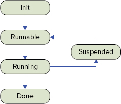
The newly created task object has to be associated with a free worker in order to actually do anything. When the worker is associated with the new task, the worker’s status is set to init. When the initial setup has been done, the status changes to runnable. At this point, the worker is ready to go but there is no free scheduler to allow this worker to run. The worker state remains as runnable until a scheduler is available. When the scheduler is available, the worker is associated with that scheduler, and the status changes to running. It remains running until either it is done or it releases control while it waits for something to be done. When it releases control of the scheduler, its state moves to suspended (the reason it released control is logged as a wait_type. When the item it was waiting on is available again, the status of the worker is changed to runnable. Now it’s back to waiting for a free scheduler again, and the cycle repeats until the task is complete.
At that point, the task is released, the worker is released, and the scheduler is available to be associated with the next worker that needs to run. The state diagram for scheduling workers is shown in Figure 5-19.
SUMMARY
This chapter introduced you to the process of query execution, including the optimization process and some of the operators used by the Query Optimizer. Then you took a look at query plans, including the different ways that you can examine them, and how to read them. Finally, you learned about the objects that SQLOS uses to manage scheduling, and how scheduling works.
Some key points you should take away from this chapter include the following:
- SQL Server uses cost-based optimization to find what it thinks is a good enough plan. This won’t always be the best plan.
- Statistics are a vital part of the optimization process.
- Many factors influence how SQL Server chooses a query plan.
- You can alter the plan chosen using a variety of plan hints and other configuration settings.