Chapter 4

Storage Systems

WHAT’S IN THIS CHAPTER?

• Storage and RAID technology
• Choosing the right storage network
• The SQL I/O system
• Windows I/O system
• Configuration best practices
• Storage performance
• Storage validation and testing

WROX.COM CODE DOWNLOADS FOR THIS CHAPTER

There are no code downloads for this chapter.

INTRODUCTION

Storage systems have been confounding database administrators and designers since Microsoft first released SQL Server. Today DBAs are not only required to design and maintain SQL Server, but are also often pressed into service as storage administrators. For DBAs working in the enterprise, communication with the server, networking, and especially storage teams are always a challenge.

This chapter will equip you, the humble database professional, with the knowledge needed to define proper storage performance. More important, you will gain insight and a common language that enables you to communicate with storage networking teams. We will follow SQL server reads and writes as they traverse the Windows and storage stacks.

By examining various storage hardware components, you will learn how best to protect your data with RAID technology. You will also see how storage area networks assist in data protection. Finally, you will learn how to validate your functional configuration and performance.

SQL SERVER I/O

Let’s begin by investigating how SQL Server generates I/O. We are concerned with reading existing data and writing new data. At its most basic SQL Server is made up of a few files that reside within the server file system. As a rule, different computer system components perform at different rates. It is always faster to process items in the CPU than it is to serve requests from processor cache. As detailed in the hardware chapter, L2 and L3 CPU cache is faster than computer memory. Server memory is faster than any I/O component.

SQL attempts to mitigate the relatively slow I/O system by caching whatever it can in system memory. Newly received data is first written to the SQL transaction log by SQL Server write-ahead logging (WAL) as you saw in Chapter 1. The data is then written to buffer pages hosted in server memory. This process ensures that the database can be recovered in the event of failure.

Storing the buffer pages in memory ensures that future reads are returned to the requestor promptly. Unfortunately, server memory is not infinite. At some point SQL server will need to write data. In Chapter 1 you learned about how SQL Server writes data to disk using the Lazy Writer and Checkpoint processes. This chapter will cover the mechanics of how the operating system and storage subsystems actually get this data onto disk storage.

Contrast these write operations with read requests that are generated by SQL Server worker threads. The workers initiate I/O read operations using the SQL Server asynchronous I/O engine. By utilizing an asynchronous operation worker threads can perform other tasks while the read request is completed. The asynchronous I/O engine depends on Windows and the underlying storage systems to successfully read and write data to permanent storage.

SQL Server takes advantage of the WriteFileGather and ReadFileScatter Win32 APIs. WriteFileGather collects data from discontinuous buffers and writes this data to disk. ReadFileScatter reads data from a file and disperses data into multiple discontinuous buffers. These scatter/gather APIs allow the bundling of potential I/O operations thus reducing the actual number of physical read and write operation.

Understanding Windows storage is the key to tuning SQL Server I/O performance and guaranteeing data integrity. This chapter aims to arm database administrators and designers with the appropriate nomenclature to enable communication with other information technology disciplines. Open, reliable communication is the ultimate key to successful relational data management.

STORAGE TECHNOLOGY

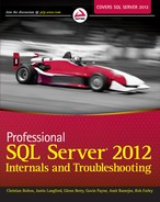
The Host Bus Adapter (HBA) handles connections from the server to storage devices and can also perform several other roles. While a basic HBA provides connectivity to storage, more advanced HBAs have embedded Array controllers. When the storage is located within or attached to the server, it is called Direct Attached Storage (DAS). A storage device managed by a dedicated external array controller is called Storage Area Network (SAN) attached storage. Figure 4-1 shows the basic building blocks of a storage subsystem.

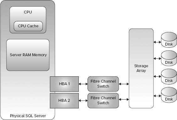
Storage devices connected to a storage network that are not logically grouped are called, rather inelegantly, a JBOD, for “just a bunch of disks (or drives).” Figure 4-2 shows an example of a JBOD. JBODs can be accessed directly by SQL Server as individual physical disk drives. Just remember that JBODs do not offer any protection against failure.

Storage array controllers group disks into volumes called a redundant array of inexpensive disks (RAID). RAID-constructed volumes offer capacity without failure protection. The simplest type of unprotected RAID set is often called disk striping, or RAID 0.

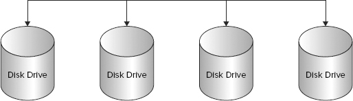
To understand a RAID 0 set, imagine a series of four disk drives lined up in a row. Data written to a stripe set will fill the first drive with a small amount of data. Each subsequent drive will then be filled with the same amount of data, at which point the process is repeated starting with the first disk drive. Figure 4-3 shows how data looks after it has been written to a RAID 0 disk subsystem. Each data stripe is made up of some uniform data size. Most RAID systems allow the user to modify the size of the data stripe.

Concatenated disk arrays are similar to stripe datasets, differing in the method used to load data. You can think of concatenated datasets as a group of disk drives that are filled in series. The first group is filled, then the second group, and so on. We will investigate the performance implications of different RAID configurations later in the Disk Drive Performance section of this chapter.

Figure 4-4 shows the contrast between striped RAID, which is serpentine in its layout, and the waterfall pattern of a concatenated disk array. Concatenated systems don’t necessarily lack data protection. Many storage arrays layer different types of RAID. One example is a system that combines mirrored physical disks into a concatenated RAID set. This combined system offers the benefits of protected data and the ease of adding more capacity on demand since each new concatenated mirror will be appended to the end of the overall RAID set.

RAID defines two ways to provide failure protection: disk mirroring and parity generation. RAID 1, often called disk mirroring, places data in equal parts on separate physical disks. If one disk fails, the array controller will mirror data from the remaining good disk onto a new replacement disk. Figure 4-5 details the frequent combination of mirroring and striping. This system is often called RAID 1 + 0 or simply RAID 10.

The storage array uses an exclusive or (XOR) mathematical calculation to generate parity data. Parity enables the array to recreate missing data by combining parity information with the data that is distributed across the remaining disks. This parity data enables you to make efficient use of your capacity but at the cost of performance, as the XOR calculation needed to generate the parity data is resource intensive. More details about the performance implications of data protection can be found in the Disk Drive Performance section of this chapter.

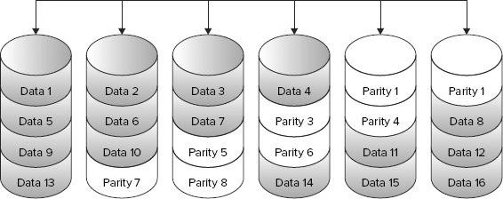
Many different parity RAID configurations have been defined. The two most common types are disk striping with parity (RAID 5) and disk striping with double parity (RAID 6). Examples of both are shown in Figure 4-6 and Figure 4-7. RAID 5 protects a system against a single disk drive failure. RAID 6 protects against a double disk failure. RAID 5 and 6 offer disk failure protection while minimizing the amount of capacity dedicated to protection. Contrast this with RAID 1, which consumes half of the available storage in order to protect the data set.

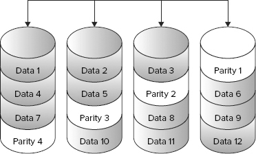
To create the parity information the RAID engine reads data from the data disks. This data is computed into parity by the XOR calculation. The parity information is written to the next data drive. The parity information is shifted to a different drive with each subsequent stripe calculation thus ensuring no single drive failure causes catastrophic data loss.

RAID 6 generates two parity chunks and diversifies each across a different physical disk. This double parity system protects against a double disk drive fault. As disk drives become larger and larger, there is a significant chance that before the failed data can be repaired a second failure will occur.

RAID 5 and RAID 6 become more space efficient on larger sets of disk drives. A RAID 5 disk set using seven data drives and one parity drive will consume less relative space than a disk set using three data drives and one parity drive.

Each of these RAID sets represents a failure domain. That is to say, failures within the domain affect the entire dataset hosted by a given failure domain. Large failure domains can also incur a performance penalty when calculating the parity bits. In a four-disk RAID 5 set, only three data drives are accessed for parity calculation. Given an eight-disk RAID set, seven drives are accessed.

You can combine RAID types into the same volume. Striping or concatenating several RAID 5 disk sets enables the use of smaller failure domains while increasing the potential size of a given volume. A striped, mirrored volume is called RAID 1+0 (or simply RAID 10). This RAID construct can perform extremely well at the cost of available capacity.

Many storage controllers monitor how RAID sets are accessed. Using a RAID 10 dataset as an example, several read requests sent to a given mirrored drive pair will be serviced by the drive with the least pending work. This work-based access enables RAID sets to perform reads more rapidly than writes. We will cover much more about the effects of RAID on I/O performance in the Disk Drive Performance section of this chapter.

SQL Server and the Windows I/O Subsystem

Microsoft SQL Server is an application that utilizes the Windows I/O subsystem. Rather than covering the minutia of how SQL Server reads and writes from the NTFS file system, we are going to explore the specific Windows I/O systems that will report errors to the Windows event logs. This should aid you in troubleshooting many storage errors.

The storage system components, shown in Figure 4-8, report errors to the Windows system Event Log. SQL Server reports errors to the Windows application log. You can either directly check the Event Logs or use System Center to scrape the Event Logs for actionable errors.

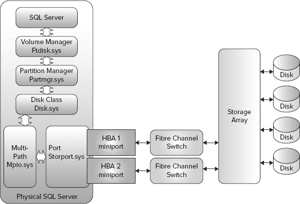
The Volume Manager driver (ftdisk.sys) creates a new I/O request packet that is passed to the Partition Manager driver (partmgr.sys). Once the request packet is created, the Volume Manager passes this packet to the Disk Class driver (disk.sys). Ftdisk.sys continues to monitor for successful delivery of the request packet. If problems are detected, then ftdisk.sys reports the errors to the system Event Log. These ftdisk errors usually represent very serious storage system issues.

At this point the Disk Class driver passes the storage request to either the Multipath System driver (mpio.sys) or the Port driver (storport.sys). Multipath I/O is a Microsoft technology that is utilized in storage area networks (SANs). Vendors can create an MPIO device-specific module (DSM) driver that details how the Multipath driver should load balance I/O across different storage pathways. Microsoft offers a generic DSM that provides limited failover capabilities. Non-SAN technologies do not use MPIO.

The HBA is the physical piece of hardware that interfaces with disk drives and other storage devices. HBA manufacturers create a miniport driver that interfaces with storport.sys. Most HBA drivers will independently report communication errors to the application Event Log.

Ideally, this entire chain of events takes no longer than 20 milliseconds. Performance is governed by a myriad of factors, the most important of which is latency. Both ftdisk.sys and SQL Server time each I/O. If the round-trip duration exceeds 15 seconds (for SQL Server or 1 minute for ftdisk.sys), then errors are reported to the SQL logs and the Windows application Event Log. As you hopefully noticed, a normal operation is measured in milliseconds, so one second is an eternity.

Choosing the Right Storage Networks

This chapter opened with an example of a SQL Server using a single disk drive. More complex storage networks link multiple hosts, or initiators, to many storage devices, or targets. These advanced storage area networks facilitate low-latency, high-throughput communication.

The storage network can facilitate the sharing of storage resources. Direct attached storage offers good performance for a relatively low cost, but DAS storage can orphan performance and capacity. Imagine several applications that grow in capacity at different rates or are used at different times. Consolidated storage that is attached to a SAN network enables users to share both storage capacity and available performance.

Complex storage networks are often built using Fibre Channel (FC) technology.

FC differs from most server network protocols in that it is not routed. Routing enables the creation of large and resilient networks, but routed networks require a lot of overhead to operate.

If you are familiar with Fibre Channel you may already be aware of routing solutions for it. Several products exist to fulfill this role; their use is extremely complex and beyond the scope of this chapter.

Because it is not routed, FC defines a standard for both direct and switched storage network connections. Modern FC networks utilize high-speed network switches to communicate.

Storage networks are not limited to Fibre Channel. Several protocols define methods for sending storage data over existing server IP networks. Fibre Channel Internet Protocol (FCIP) allows Fibre Channel data frames to be encapsulated within an IP packet. Internet Small Computer Systems Interface (iSCSI) allows the transmission of SCSI data over IP networks.

FCIP and iSCSI transport different layers of the storage network. Fibre Channel frames are analogous to Ethernet data frames. SCSI is a storage control system comparable to Internet Protocol. Transmission Control Protocol is an Internetworking protocol and therefore has no analogue in storage networking. Emerging technologies such as Fibre Channel Over Ethernet (FCOE) combine the attributes of existing Fibre Channel networks with Ethernet routed networks.

Regardless of the specific network technology that is used to transport storage traffic, keep in mind that bandwidth is not infinite. Excessive storage traffic not only negatively impacts the performance of a single system, it can hamper all connected components. Many applications must meet minimum performance requirements spelled out in service-level agreements (SLAs). Storage network performance is critical to overall application performance.

Block-Based Storage vs. File-Based Storage

The operating system, in this case Windows, uses NTFS to create a structure that enables it to use one or more blocks to store files. When a server accesses a physical disk directly, it is called block-based access. When data is accessed over a server network, such as TCP/IP, it is called file data. Devices that provide file access are called network-attached storage (NAS).

Disk drives store data in blocks. Each block contains 512 bytes of data (some storage arrays use 520-byte blocks — the extra 8 bits define a checksum used to guarantee data integrity).

Disk drive data blocks are individually numbered by the disk firmware in a scheme using what are called logical block numbers (LBNs).

Starting with SQL Server 2008 R2, storage administrators have the option of using Server Message Block (SMB) networks to access data files. Technet offers a detailed overview of the advantages of SMB here: http://technet.microsoft.com/en-us/library/ff625695(WS.10).aspx.

SQL Server 2012 supports SMB version 3.0 which offers improved performance over earlier versions. For more information on configuring SQL Server 2012 with SMB 3.0 visit: http://msdn.microsoft.com/en-us/library/hh759341.aspx.

Setting up an SMB network enables you to connect to your file over a UNC path (\server_name share). This access can greatly simplify the setup of network-based storage, although you should use caution and specifically check to ensure that your particular system is supported, as NAS devices often are not supported for use in this configuration.

Contrast SMB with the use of an iSCSI network. iSCSI is a protocol used for accessing block data over a server network. It requires the use of initiator software on the host server and a compatible iSCSI storage target.

Both SMB and iSCSI utilize a server network to communicate. You must ensure that the server network is low latency and has the bandwidth available to handle the demands that will be placed on it by either technology. Most Fibre Channel networks are dedicated to handling only storage traffic.

If you utilize a server network to transport block or file SQL Server traffic, it may need to be dedicated to transferring only the storage traffic. In lieu of dedicated networks, consider implementing Quality of Service (QoS) that puts a higher priority on storage traffic over normal network packets.

Keep in mind that no technology provides a magic bullet. Even robust networks can be filled with traffic. Storage transfers are extremely sensitive to delay.

Shared Storage Arrays

Shared array controllers are primarily responsible for logically grouping disk drives. Sharing the storage controller enables the creation of extremely large volumes that are protected against failure. In addition to the normal features of direct attached storage controllers, a shared array controller provides both storage performance and capacity.

Shared array controllers, often called SAN controllers, offer more advanced features than direct attached systems. The feature sets are divided into three categories:

• Efficient capacity utilization
• Storage tiering
• Data replication

Before diving into the features of SAN arrays, however, it would be helpful to look at some of the language that storage administrators use to describe their systems.

Capacity Optimization

It has been our experience that most information technology professionals are not very good at predicting the future. When asked how much performance and space they anticipate needing over the next three to five years, administrators do their best to come up with an accurate answer, but unfortunately real life often belies this estimate.

Meet Bob. Bob forecasted that his new OLTP application would start at 10GB and grow at 10GB per year over the next five years. Just to be on the safe side, Bob asked for 100GB in direct-attached storage. Bob’s new widget sells like hotcakes and his database grows at 10GB per month. Seven months in, Bob realizes that he is in trouble. He asks his storage administrators for another 500GB in space to cover the next five years of growth.

Unfortunately, the storage and server administrators inform Bob that other users have consumed all the space in his data center co-location. The information technology group is working diligently to expand the space, but it will be six months before they can clear enough space to accommodate his storage. Bob notes that never again will he come up short on storage and go through the pain of expanding his system.

Moving forward Bob always asks for 10 times his original estimate. In his next venture Bob finds that his database will also grow at 10GB per year over 5 years but this time Bob, having “learned his lesson” asks for 10GB a month. Unfortunately Bob’s actual storage requirement was closer to 5GB per year.

Bob has unwittingly become his own worst enemy. When Bob needs storage for his second application there isn’t any storage available because Bob is simultaneously holding on to unused storage for his first application. He has underprovisioned his storage requirements for his second application while massively overprovisioning his first.

Bob’s example is not unique. IT shops the world over consistently overprovision storage. Imagine the implications; over the life of the storage and server, companies purchase a significant amount of excess storage that requires powering and servicing. To combat this wasteful use of space, several storage array manufacturers now sell a technology called thin provisioning.

Thin provisioning uses the concept of just-in-time storage allocation within storage pools, whereby many physical disk drives are amalgamated into one large pool. Appropriate RAID protection is applied to the disk drives within the pool. Many volumes can be created from each pool. Synthetic or virtual volumes are presented to the host servers.

When a volume is created as a thin device it allocates only a minimum amount of storage. From the perspective of the operating system, the volume is a certain set size, but the actual data usage within the thin pool closely matches the size of written data. As new data is written to the volume, the storage array allocates more physical storage to the device. This enables the storage administrator to directly regulate the amount of storage that is used within the storage environment.

Because over-forecasting is no longer under-utilizing space, the database administrator can focus on easing operational complexity, versus trying to optimally forecast storage. Creating a single data file within a file group and later adding files while maintaining performance is an extremely painful operation. If a database is built without planning for growth and instead is concatenated over time by adding files, then data access is not uniform.

One possible growth-planning solution is to create several data files on the same volume. If that volume becomes full, the original data files can be moved. This data file movement will require downtime, but it is preferable to reloading the entire dataset. When utilizing storage pools it is possible to create large thin volumes that may never be fully utilized. This is possible because the storage systems are provisioning storage only as it is needed. Many SAN array controllers also facilitate online volume growth.

Unfortunately, many DBAs subvert the concept of thin provisioning by fully allocating their database at creation time. Most database administrators realize that growing a data file can be a painful operation, so they often allocate all the space they will ever need when the database is created. Unfortunately, for our thin pool, SQL Server allocates data and log files by writing zeros to the entire data file.

If the Windows Server is set to use instant file initialization, the file will be created in a thin-pool-friendly way. New storage will be allocated in the pool only as the data actually increases (http://msdn.microsoft.com/en-us/library/ms175935(v=SQL.105).aspx). The DBA can also ensure that the file is thin-pool-friendly by creating data and log files that are only as large or slightly larger than the data the file will contain.

If the data file has already been created as a large file filled with zeros, then a feature called Zero Page Reclaim can be used on the array to reclaim the unused space. Running Zero Page Reclaim allows the array to return the zero space to the available storage pool so it can be allocated to other applications.

Deleting data from within a database or even deleting files from a volume will not return free space to the thin storage pool. In the case of reclaiming deleted file space, most storage vendors offer a host-side tool that checks the NTFS Master File Table and reallocates space from deleted space. If you decided to delete space from within a SQL Server data or log file you need to run the DBCC SHRINKFILE command to first make the file smaller, and then run the host-side storage reclamation tool to return space to a given thin pool.

Unfortunately, thin storage pools have a dirty little secret. In order to optimize storage use in a world where storage forecasting is an inexact science, it is necessary to overprovision the thin pools. This means that storage teams must closely monitor the growth rate at which new storage is being used.

Storage Tiering

Non-volatile storage is generally manufactured to offer either high performance or high capacity. High-performance disk and flash drives are much more costly than high-density storage. In an effort to make the most efficient use of both capacity and performance, SAN arrays allow several types of storage to be mixed within a given array.

Our database administrator, Bob, is now stinging after submitting his budget to his manager, Stan. Bob needs to come up with a plan for reducing his storage requests for the next fiscal year. He bumps into Eddy, who works for Widget Company’s storage department, at the water cooler.

Eddy has heard of Bob’s plight and suggests that Bob place his backup files on less costly high-capacity SATA drives. This will reduce Bob’s budget request and make Stan happy. Bob will keep his log and tempdb files on higher-performance SAS RAID 10 volumes and shift his data files onto less expensive RAID 5 SAS drives.

Because the server is tied to a storage network, the different tiers of disks don’t even need to exist within the same array. Bob could place his data, log, and tempdb files on one array and move his backup data to a completely different storage system. This approach offers the added benefit of shrinking the possible failure domain. If the primary array suffers a catastrophic failure, the backup data still exists on a separate array.

This mixing and matching of storage within a SAN array is called storage tiering. Some storage arrays provide automated storage tiering, monitoring volumes or pieces of volumes for high performance. When predetermined performance characteristics are detected, the array will migrate data onto a higher tier of storage. Using this model, Bob only needs to put all his data on a storage volume; the array determines where to place the data and when to move it.

Different storage vendors have implemented storage tiering in unique ways. One of the most unique features is the granularity of data that is migrated. Some arrays use a transfer size of a few kilobytes. Other arrays migrate gigabytes of data. Each system offers different performance. Be sure to evaluate any potential system to ensure it meets your needs.

Data Replication

SAN arrays offer both internal and external storage data replication. Internal replication consists of data snapshots and clones. Some storage arrays offer inner array data migration features. Both a snapshot (also called a snap) and a clone offer a point-in-time data copy. This data copy can be used for backup or reporting.

Both snapshots and clones need to be created in sync with the database log and data files. In order to maintain SQL data integrity, both the log file and data files need to be copied at exactly the same time. If the log and data files are not in sync, the database can be rendered unrecoverable.

Prior to creating the point-in-time data copy, you need to decide on the type of SQL Server recovery that is needed. You can create application-consistent copies using the SQL Server Virtual Backup Device Interface (VDI). VDI is an application programming interface specification that coordinates the freezing of new write operations, the flushing of dirty memory buffer pages to disk (thus ensuring that the log and data base files are consistent), and the fracturing of the clone or snap volume. Fracturing is the process of stopping the cloning operation and making the snapshot or clone volume ready for use. Once the fracture is complete, the database resumes normal write operations. Reads are not affected.

Crash-consistent data copies depend on the fact that SQL Server uses a write-ahead logging model, as described earlier. New data is first written to the disk or storage volume. As soon as the write operation is complete, it is acknowledged. Only after the data has been successfully written and acknowledged will SQL Server write data to its buffer pool.

If the database is shut down before it has a chance to flush dirty buffer-page data to disk, the write-ahead logging feature enables SQL Server to recover data that was written to the log but not to the database files. This recovery model enables the use of advanced replication technologies.

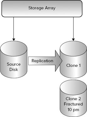
Clone data volumes create an exact replica of the source volume as of the point in time when the clone was created (Figure 4-9). Because the clone is an exact copy it enables the isolation of I/O performance. The source volume can continue to operate normally while the clone can be mounted to a different host. This enables a workload to be distributed among many machines without affecting the source volume. Such a scenario is extremely useful to enable high-performance reporting systems. Keep in mind that the clone volume requires the same amount of space within the storage array as the original volume requires.

A hardware storage snapshot, shown in Figure 4-10, is a point-in-time data copy. The snapshot differs from a clone data copy in that it keeps only the original copy of changed data.

When a change is written to the storage volume, the array stores the original data and then writes the new data to disk. All the changes are tracked until the user requests a point-in-time data copy. The array correlates all the changed data blocks that now represent the state of the volume at that moment in time.

The user can continue to create as many snap volumes as the array supports. Snapshots utilize capacity based on the rate of data change. It is possible to churn so much data that the snapshots consume more data than the actual data volume. Expiring snap volumes can reduce the amount of space consumed.

Snapshots do not isolate performance. Any I/O executed against the snap volume is accessing both the source volume and any saved changes. If the primary database server is so busy that you have decided to utilize a second server that performs reporting functions, a clone volume may be a better choice than a snapshot.

For business continuance and disaster recovery (BCDR) you could also consider a layered approach. The clone volume will provide a unique data copy. Keep in mind that the clone is a mirror of the original data and will consume the same capacity as the original volume. Keeping several clone copies can be cost prohibitive. Snapshots can offer many inexpensive point-in-time copies, but they won’t work if the primary data volume is compromised. You can enable a data clone to protect against a catastrophic data failure. The snapshots can be taken much more frequently and enable the DBA to roll back to a specific point in time (which is extremely useful in case of user error or computer virus).

Remote Data Replication

Both SAN and NAS array controllers offer external data replication. This feature enables two or more array controllers to synchronize data. Vendors provide either a real-time or a point-in-time data migration framework.

Real-time frameworks replicate changes as they are written to the array. This replication is performed synchronously or asynchronously. Synchronous data replication is extremely sensitive to latency and is therefore not used over great distances.

Synchronous Replication

When SQL Server writes changes to either the data or the log, remember that both the user database and the log files must be replicated; a synchronous replication system writes the I/O to its battery-backed data cache. The array then sends the I/O to its replication partner. The partner writes the I/O to its own cache and then sends a successful acknowledgment to the source array.

At this point, based on proprietary caching algorithms, the storage arrays write the data from their cache to disk, and a success acknowledgment is sent to the SQL Server. As you can see, this process adds latency to the entire write process. Distance directly translates to latency. If the systems are asked to handle too much replicated data, or are placed too far apart, the database will slow considerably.

Asynchronous Replication

Rather than wait for a single change to be committed to both arrays, asynchronous replication sends a stream of changes between the arrays. As I/O is successfully written to cache, the source array returns a success acknowledgment to SQL Server. This way, changes are written without slowing the SQL Server processes.

The primary array sends changes to the remote array in a group. The remote array receives the group of changes, acknowledges the successful receipt, and then writes the changes to physical media. Each vendor offering asynchronous remote replication has a property method for ensuring successful delivery and recovering from communication issues between the arrays.

From a BCDR prospective, the drawback to implementing asynchronous replication is the potential for some data loss. Because the write I/O is instantly acknowledged on the source array, some amount of data is always in transit between the arrays. Most unplanned failover events will result in transit data being lost. Due to the design of SQL server lost data does not mean that the remote database is corrupt.

Several storage vendors combine point-in-time technology with remote replication. These features enable the administrator to take a clone or snapshot of the user databases (using VDI to create an application-consistent data copy if desired) and send the data to a remote array.

As with asynchronous replication, point-in-time remote replication offers the advantage of low server impact. Remotely sending a snapshot enables you to specifically control the potential for data loss. If you set the snap interval for five minutes, you can be reasonably certain that in the event of unplanned failure you will lose no more than five minutes of changes. Identifying an exact amount of expected data loss can offer huge advantages when negotiating the parameters of BCDR with the business.

Windows Failover Clustering

Many SQL Server installations utilize Windows Failover Clustering to form high-availability SQL Server clusters. These systems create a virtual SQL Server that is hosted by an active server and at least one passive server. SQL Server 2008 and 2008 R2 failover clusters supported only shared storage failover clustering. The SAN storage array allows all SQL Server clusters to access the same physical storage and move that storage between nodes.

SQL Server failover clusters are based on the concept of “shared nothing”; the SQL Server instance (or instances) can live on only one active server. SQL Server places an active lock on log and data files, preventing other servers or programs from accessing the files. This is incorporated to prevent data changes that SQL Server would have no way to detect. In addition to file locks, the failover cluster also actively prevents other systems from using the storage volumes by using SCSI reservation commands.

Failover clustering can be set to automatically fail the instance over to a standby server when a failure occurs. SQL Server failover clusters also support the use of geo-clustering. A geo-cluster uses storage replication to ensure that remote data is in-sync with the source data. Storage vendors provide a proprietary cluster resource dynamic link library (DLL) that facilitates cluster-to-storage-array communication.

The use of a resource DLL enables a rapid failover between sites with little or no administrator involvement. Traditional failover systems require the interaction of many teams. Returning to our example, assume that Widget Company has just implemented a local SQL Server with a remote failover system.

The system in use by Widget uses traditional storage replication. When the Widget DBAs try to execute a failover they first need to contact the storage administrators so they can run failover scripts on the storage arrays. Once the storage is failed to the remote site, the DBAs can bring the database online. Because the server name is different, the DBAs need to reconfigure the database to do that. Now the application owners need to point all the middle-tier systems to the new server.

Even when the failover is planned it is extremely resource intensive to implement. The use of a geo-cluster greatly simplifies the failover process. The failover is implemented automatically whenever the SQL Server geo-cluster is failed over to a remote node. Unfortunately, SQL Server 2008 and 2008R2 only supported geo-clustering when both servers shared the same IP subnet.

This networking technology is called a stretch virtual local area network, or stretch VLAN. The stretch VLAN often requires that network engineers implement complex networking technologies. SQL Server 2012 solves this through AlwaysOn Failover Cluster Instances. This new feature enables each SQL Server to utilize an IP address that is not tied to the same IP subnet as the other hosts.

SQL Server AlwaysOn Availability Groups

The configuration and setup of AlwaysOn Availability Groups is beyond the scope of this chapter. From a storage perspective, Availability Groups offer a new, server-based method for replicating data that is application centric rather than platform centric. As discussed earlier, storage systems can use point-in-time data copies to facilitate data backup and performance isolation. Deciding between application based failover and hardware based failover is an architecture choice.

Earlier versions of SQL Server utilized log shipping, and later SQL Server mirroring, to keep standby SQL Servers updated with information. In the case of both log shipping and storage replication, the remote database must be taken offline prior to data synchronization. Availability Groups enable the use of near-real-time readable secondary database servers.

The read-only data copy can facilitate reporting offload or even backup. In addition, Availability Groups support synchronous or asynchronous data replication and also multiple secondary servers. You can configure one secondary as a reporting system that is hosted locally, and a second server can be hosted remotely, thus providing remote BCDR.

From a storage perspective, note the following caveats: Each remote secondary server needs as much storage capacity (and usually performance) as the primary database. In addition, it is critical that your network infrastructure is designed to handle the increased network traffic that can be generated by replicating data locally and remotely. Finally, all your servers must have enough performance available to handle the replication. If your server is already processor, storage, or memory bound, you are going to make these conditions worse. In these cases it is often advantageous to enable storage-based replication. Think of AlwaysOn Availability Groups as a powerful new tool that now enhances your SQL Server toolkit.

Risk Mitigation Planning

All of the replication and backup technologies described here are designed to mitigate risk. To properly define the specific procedures and technologies that will be used in your BCDR strategy, you need to decide how soon you need the system online and how much data your business is willing to lose in the process.

The projected time that it will take to bring a failed system online is called the recovery time objective (RTO). The estimated amount of original data that may be lost while the failover is being executed is called the recovery point objective (RPO). When designing a recovery plan it is important to communicate clear RTO and RPO objectives.

Ensure that the recovery objectives will meet business requirements. Be aware that systems that provide a rapid failover time with little or no data loss are often extremely expensive. A good rule of thumb is that the shorter the downtime and the lower the expected data loss, the more the system will cost.

Let’s look at an example failover system that has an RTO of 1 hour and an RPO of 10 minutes. This imaginary system is going to cost $10,000 and will require DBAs to bring up the remote system within one hour. If we enhance this example system to automatic failover it will reduce our RTO to 10 minutes, and we should not lose any data with an RPO of 0. Unfortunately, this system will cost us half a million dollars.

MEASURING PERFORMANCE

The single most important performance metric is latency. Latency is a measure of system health and the availability of system resources. Latency is governed by queuing theory, a mathematical study of lines, or queues. An important contribution to queuing theory, now known as Little’s Law, was introduced in a proof submitted by John D. C. Little (http://or.journal.informs.org/content/9/3/383) in 1961.

Put simply, Little’s Law states that given a steady-state system, as capacity reaches maximum performance, response time approaches infinity. To understand the power of Little’s Law, consider the typical grocery store. If the store only opens one cash register and ten people are waiting in line, then you are going to wait longer to pay than if the store opened five or ten cashiers.

Storage systems are directly analogous to a grocery store checkout line. Each component has a certain performance maximum. Driving the system toward maximum performance will increase latency. We have found that most users and application owners directly correlate latency with failure. For example, it won’t matter that a payroll system is online if it can’t process transactions fast enough to get everyone’s paycheck out on time.

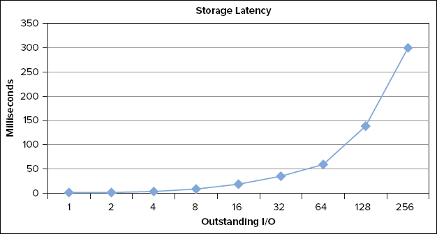
You test I/O performance using several tools that are described later. You test storage using a logarithmic scale, starting with one I/O, moving to two, then four, then eight, and finally peaking at 256 I/Os that are all sent to storage in parallel (see Figure 4-1). As it turns out, this test perfectly demonstrates Little’s Law by defining how storage operates.

As you can see in Figure 4-11 the storage response time remains less than our goal of 10 milliseconds through eight outstanding I/Os. As we increase the workload to 16 outstanding I/Os, the latency increases to 20 milliseconds. We can determine from this test that our configuration is optimal when we issue between 8 and 16 I/Os. This is called the knee of the curve. The system is capable of a lot more work, but the latency is higher than our tolerance.

The remainder of this chapter explores how to accurately measure performance and latency. Techniques for establishing performance baselines are demonstrated, and then you will examine how the application of advanced storage pooling technology is changing how database systems are designed.

Storage Performance Counters

Windows Performance Monitor (perfmon) allows Windows Server users to capture storage performance metrics. For the purposes of storage monitoring, you utilize the LogicalDisk performance monitor object. Both logical and physical disk counters deliver storage performance metrics. The logical disk counters show the performance of a specific partition, while the physical disk counters cover the entire LUN (a Logical Unit Number is a term that describes a storage volume that is hosted by a storage controller). Table 4-1 shows a list of the available Windows storage performance counters.

TABLE 4-1: Windows Storage Performance Counters

LOGICALDISK PERFMON OBJECT
Average Disk sec/Read
Average Disk sec/Write
Disk Reads/sec
Disk Writes/sec
Disk Read Bytes/sec
Disk Write Bytes/sec

The Average Disk Sec/Read and Write counters measure the time it takes for an input output (I/O) operation to be sent from the server to the storage system and back. This latency measure is the single biggest indicator of I/O system health. Reads and writes are treated separately because most storage systems perform one operation faster than the other. If you are using a storage array with a battery-backed cache, it will often write in just a few milliseconds, whereas a random read will take longer.

The latency counters are measured in milliseconds. A reading of 0.001 is one millisecond, 0.010 is 10 milliseconds, and .100 is 100 milliseconds. SQL Server best practices call for latency that is under 20 milliseconds. This is not a hard-and-fast rule, however, as many applications will not tolerate latency that exceeds several milliseconds.

It is important to understand the underlying hardware configuration, application, and workload. In some cases, such as a SQL Server standard backup, large I/O sizes will drastically increase latency. If you change the backup I/O size to 8MB, the latency will increase, but you can still achieve a lot of work.

If you are implementing a specialized system, such as a SQL Server Fast Track Data Warehouse, you will actively configure the data files so they issue sequential I/O. Be sure to test your specific configuration so you can properly interpret the results.

The Disk Reads and Writes per second counters list how many I/Os are generated each second (Storage administrators often refer to this as IOPS). Disk Read and Write Bytes per second demonstrate the throughput of your storage system. To calculate average I/O sizes, simply divide bytes per second by the number of operations per second.

Knowing the size of the I/O can reflect application behavior. When performing highly random I/O access, SQL Server will write 8K data pages and read 64KB data extents from the data files. Performing sequential operations, such as a table scan, will generate I/O that is dynamically sized from 8K to 512KB. Dynamic I/O sizing, also known as Read-Ahead, is one of the hidden gems of SQL Server. Increasing I/O size decreases the number of I/Os and increases efficiency.

Disk Drive Performance

A disk drive (see Figure 4-12) is made up of an external logic board and an internal hard drive assembly. The logic board provides connectivity between the disk and the host. Each drive interface supports one of many available communications protocols. Modern interfaces use a high-speed serial connection. The interfaces that are most commonly used for database applications are SATA (Serial Advanced Technology Attachment), FC (Fibre Channel), and SAS (Serial Attached SCSI).

The hard drive assembly is serviceable only inside a high-technology clean room. Opening the cover on a hard disk drive will void the warranty. The drive platter rotates around a spindle and is powered by a spindle motor. A drive is made up of several platters that are stacked. Each platter is double-sided and coated with a magnetic oxide.

Data is physically read and written by a hard drive head. Each drive platter has a dedicated drive head. An actuator arm houses all the drive heads, and a magnetic actuator moves the arm. You can think of a hard drive as a record player. The platter spins and the head reads and writes data. Unlike a record player, however, the disk drive head can move back and forth. The head actually rides just above the disk surface on a cushion of high-pressure air that is created when the platter spins at high speed.

SATA disk drives provide commodity storage. They offer much larger capacity than FC or SAS drives. At the time of this writing, SATA drives are available with a capacity of three terabytes (3TB). SATA drives spin at lower speeds — 5,400 to 7,200 RPM. They are sold for both the consumer and the enterprise markets. Enterprise drives are designed for more continuous use and higher reliability.

Both FC and SAS drives are considered enterprise-class disk drives. They are available in 7,200, 10,000, and 15,000 RPM models. With the exception of Nearline SAS (NL-SAS) drives, these disk drives are generally lower in capacity than SATA disk drives. SAS 6GB/s drives are displacing Fibre Channel 4GB/s drives in the marketplace.

Modern SAS drives are manufactured in a 2.52 form factor, unlike the traditional 3.52 form factor of Fibre Channel and SATA drives. This smaller drive enables more disk drives to be housed in a given space. NL-SAS drives offer a high-reliability enterprise SATA drive with a SAS interface.

The logic board governs how the disk operates. Each disk contains buffers, and some disk drives contain cache. For the proper operation of SQL Server write-ahead logging, volatile cache must be bypassed for write operations. Most array vendors will guarantee cached data with battery backing. When using disks directly in a JBOD, it is important to ensure that they meet SQL Server reliability requirements.

A disk drive is made of both electronic and mechanical components. When data is read sequentially, the drive can read it as fast as the drive spins. When the data needs to be accessed out of order, the head needs to move to the appropriate track. Head movement, or seeking, is not instantaneous.

A sequential read consists of a head movement followed by the sequential reading or writing of data. When data is not sequentially located, the disk drive executes a series of random operations. Random access patterns are much slower because the head needs to physically move between tracks.

Drive manufacturers provide a measurement called maximum seek time that reflects how long it will take for the drive head to move from the innermost tracks to the outermost tracks. The manufacturer also provides what is known as average seek time, the average time it will take to move the drive head to any location on the disk.

Disk Drive Latency

You can calculate the time it takes to move the head to a location on the disk mathematically. The number of times a disk can rotate in a millisecond limits the amount of data the drive can generate, a limitation called rotational latency. To calculate how many random I/Os a hard disk can perform, the following equation is used:

This equation works by normalizing all calculations to milliseconds. To find IOPS, you start by dividing 60,000 (because there are 60,000 milliseconds in a minute) by the hard disk rotations per minute. Dividing the revolutions per millisecond by 2 accounts for the fact that the head needs to exit the first track and enter the second track at specific points, requiring about two rotations. You add the revolutions result to the seek time and convert the result back to seconds by dividing 1,000 by this sum.

For example, consider a 10,000-RPM disk. This drive will rotate about 6 times per second. You account for the fact that it will take your drive two rotations to move between tracks and then add the seek time. This drive has a read seek time of 4 milliseconds. Dividing 1,000 by 7 results in 143 I/Os per second:

We have tested many drives over the years and this formula has proven reliable. Remember that each individual model of disk drive varies. Having said that, you can calculate IOPS for the most frequently used disk drives:

If you need more IOPS, then simply add more disks. If one disk will perform 150 IOPS, then two will perform 300. When you need 10,000 IOPS, you only need 54 physical disks. If you actually want to keep the data when one of the drives fails, then you need 108 disks. Those 108 disks will provide 10,000 IOPS when the database needs to read, but only 5,000 IOPS for writes. RAID causes overhead for both space and performance. RAID 1+0 is fairly easy to calculate. You will receive N number of reads and N divided by 2 writes. RAID 5 is much trickier to calculate.

To generate the parity information, a RAID controller reads relevant data and performs an XOR calculation. Let’s take a small RAID set of four disks as an example. One write operation will generate two writes and two reads. We are assuming that there are two existing data chunks and we are writing the third. We need to write the resultant parity and the new data block.

RAID controllers vary greatly in design, but generally speaking, they utilize their internal cache to assist in the generation of parity information. Typically, Raid 5 enables N number of reads and N divided by 4 writes.

RAID 6 protects against double disk failure and therefore generates double the parity. An 8-disk RAID set consists of two parity chunks and six data chunks. You need to write the new data chunk and two parity chunks, so you know that you have three writes. You need to read the other five data chunks, so you are looking at eight operations to complete the RAID 6 write. Luckily, most RAID controllers can optimize this process into three reads and three writes.

Table 4-2 provides a guide to calculating common RAID overhead. Please remember that each system is different and your mileage may vary.

TABLE 4-2: RAID Overhead

RAID TYPE	READ	WRITE
0	N	N
1+0	N	N ÷ 2
5	N	N ÷ 4
6	N	N ÷ 6

Sequential Disk Access

Microsoft SQL Server and various hardware manufacturers partner to provide guidance for data warehouse systems. This program is called SQL Server Fast Track Data Warehouse. A data warehouse system is designed to hold a massive amount of data. The Fast Track program takes great care to design storage hardware that is perfectly sized for a specific server platform.

The data warehouse is architected such that data is sequentially loaded and sequentially accessed. Typically, data is first loaded in a staging database. Then it is bulk loaded and ordered so that queries generate a sequential table access pattern. This is important because sequential disk access is far more efficient than random disk access. Our 15,000-RPM disk drive will perform 180 random operations or 1,400 sequential reads. Sequential operations are so much more efficient than random access that SQL Server is specifically designed to optimize sequential disk access.

In a worst-case scenario, SQL Server will read 64KB data extents and write 8K data pages. When SQL Server detects sequential access it dynamically increases the request size to a maximum size of 512KB. This has the effect of making the storage more efficient.

Designing an application to generate sequential disk access is a powerful cost-saving tool. Blending sequential operations with larger I/O is even more powerful. If our 15,000-RPM disk performs 64KB random reads, it will generate about 12MBs per second. This same drive will perform 88MBs per second of sequential 64KB reads. Changing the I/O size to 512KB will quickly cause the disk drive to hit its maximum transfer rate of 600MBs per second.

Increasing the I/O size has its limitations. Most hardware RAID controllers are designed to optimally handle 128KB I/Os. Generating I/Os that are too big will stress the system resources and increase latency.

One example is a SQL Server backup job. Out-of-the-box, SQL Server backup will generate 1,000KB I/Os. Producing I/Os this large will cause a lot of stress and high latency for most storage arrays. Changing the backup to use 512KB I/Os will usually reduce the latency and often reduce the time required to complete the backup. Each storage array is different, so be sure to try different I/O sizes to ensure that backups run optimally.

Henk Van Der Valk has written several articles that highlight backup optimization:

http://henkvandervalk.com/how-to-increase-sql-database-full-backup-speed-using-compression-and-solid-state-disks
 
http://henkvandervalk.com/how-to-increase-the-sql-database-restore-speed-using-db-compression-and-solid-state-disks

This Backup statement will set the maximum transfer size to 512KB.

BACKUP DATABASE [DBName] TO  DISK = N'E:dumpBackupFile.bak'
WITH MAXTRANSFERSIZE=524288,  NAME = BackupName
GO

Server Queues

Each physical disk drive can perform one operation and can queue one operation. Aggregating disks into a RAID set increases the pool of possible I/O. Because each physical disk can perform two operations, a viable queue setting is determined by multiplying the number of disks in a RAID set by two. A RAID set containing 10 disk drives, for example, will work optimally with a queue of 20 outstanding I/Os.

Streaming I/O requires a queue of I/Os to continue operating at a high rate. Check the HBA settings in your server to ensure they are maximized for the type of I/O your application is generating. Most HBAs are set by the manufacturer to a queue of 32 outstanding I/Os. Higher performance can often be achieved by raising this value to its available maximum. The SQL Server FAST Track program recommends that queue depth be set at 64.

Keep in mind that in a shared storage SAN environment, the performance gains of one application are often achieved at the cost of overall performance. As a SQL Server administrator, be sure to advise your storage administrators of any changes you are making.

File Layout

This section divides the discussion about how to configure storage into traditional disk storage and array-based storage pools. Traditional storage systems offer predictable performance. You expect Online Transaction Processing (OLTP) systems to generate random workload. If you know how many transactions you need to handle, you can predict how many underlying disks will be needed in your storage array.

For example, assume that you will handle 10,000 transactions, and your storage is made up of 10K SAS drives that are directly attached to your server. Based on the math described earlier, you know that a 10K SAS drive will perform about 140 IOPS; therefore, you need 142 of them. Seventy-one disks would be enough to absorb 10K reads, but you are going to configure a RAID 1+0 set, so you need double the number of disks.

If you need to handle a lot of tempdb operations, then you need to appropriately size the tempdb drive. In this case, you are going to design tempdb to be about 20 percent of the expected I/O for the main data files, so you expect 2,000 IOPS. This will require that 28 disks in a RAID 1+0 configuration back the tempdb database.

You expect that a backup load will be entirely sequential in nature. Remember that SATA drives perform sequential operations extremely well, so they are a great candidate for dump drives. These drives are usually less expensive and offer greater capacity than SAS or Fibre Channel disks.

Large SATA disks store data in an extremely dense format, which puts them at greater risk for a failure and at the same time increases the chance that a second failure will occur before the RAID system can regenerate data from the first failure. For this reason, RAID 6 is an ideal candidate to protect the data drives. RAID 6 has the greatest performance overhead, so it is important to adjust the backup I/O appropriately. In most cases backup I/O should not exceed a 512KB transfer size.

Finally, you need to plan for your log drives. Logs are extremely latency sensitive. Therefore, you should completely isolate the log onto its own set of RAID 1+0 SAS disk drives. You expect sequential I/O, so the number of disks is governed by capacity rather than random performance I/O.

Why wouldn’t you mix the log drive with the backup drive? Sequential disk access assumes that the drive head enters a track and reads sequential blocks. If you host applications that sequentially access a set of disk drives, you will cause the disk drive head to seek excessively.

This excessive head seeking is called large block random access. Excessive seeking can literally drop the potential IOPS by half:

Isolating sequential performance not only applies to log files. Within a database you can often identify specific data tables that are sequentially accessed. Separating this sequential access can greatly reduce the performance demand on a primary storage volume.

In large databases with extremely heavy write workloads, the checkpoint process can often overwhelm a storage array. SQL Server checkpoints attempt to guarantee that a database can recover from an unplanned outage within the default setting of one minute. This can produce an enormous spike of data in an extremely short time.

We have seen the checkpoint process send 30,000 write IOPS in one second. The other 59 seconds are completely idle. Because the storage array will likely be overwhelmed with this workload, SQL Server is designed to dial back the I/O while trying to maintain the one-minute recovery goal. This slows down the write process and increases latency.

In SQL Server 2008 and 2008 R2, you can start SQL Server with the –k command-line option (–k followed by a decimal representing the maximum MB per second the checkpoint is allowed to flush). This option can smooth the impact of a checkpoint at the potential risk of a long recovery and changed writing behavior. SQL Server 2012 includes a new feature called Indirect Checkpoint. The following Alter Database statement will enable Indirect Checkpoint:

ALTER DATABASE <Database_Name>
SET TARGET_RECOVERY_TIME = 60 SECONDS

Indirect Checkpoint has a smoothing effect on the checkpoint process. If the system would normally flush 30K IOPS in one second, it will now write 500 IOPS over the one-minute recovery interval. This feature can provide a huge savings, as it would take 428 10K disks configured in a RAID 1+0 stripe to absorb the 30,000 I/O burst. With Indirect Checkpoint you can use only eight disks. As with any new database feature, ensure that you fully test this configuration prior to turning it loose in a production environment.

Many organizations use shared storage arrays and thin storage pools to increase storage utilization. Keep in mind that storage pools amalgamate not only capacity, but also performance. We have previously recommended that data, log, backup, and temporary database files be isolated onto their own physical storage. When the storage is shared in a storage pool, however, this isolation no longer makes sense.

The current reason for separation is to protect the data, diversifying it across failure domains. In other words, don’t keep all your eggs in one basket. It is advisable to ensure that database backups and physical data reside on different storage groups, or even different storage arrays.

Many IT groups maintain separate database, server, networking, and storage departments. It is important that you communicate the expected database performance requirements to the storage team so they can ensure that the shared storage arrays are designed to handle the load.

Once your application is running on a shared thin storage pool, performance monitoring is critical. Each of the applications is intertwined. Unfortunately, many systems are active at the exact same time — for example, end of month reporting. If your application negatively impacts other applications, it is often more beneficial and cost effective to move it out of the shared storage environment and onto a separate system.

Partition Alignment

Windows versions prior to Windows Server 2008 did not properly align Windows Server partitions to the underlying storage geometry. Specifically, the Windows hidden sector is 63KB in size. NTFS allocation units default to 4K and are always divisible by 2. Because the hidden sector is an odd size, all of the NTFS allocation units are offset. This results in the possibility of generating twice the number of NTFS requests.

Any partition created using the Windows 2008 or newer operating systems will automatically create sector alignment. If a volume is created using Windows 2003 or older operating systems, it has the possibility of being sector unaligned. Unfortunately, a misaligned partition must be recreated to align it properly.

For more information on sector alignment, please see this blog post: http://sqlvelocity.typepad.com/blog/2011/02/windows-disk-alignment.html.

NTFS Allocation Unit Size

When formatting a partition you are given the option to choose the allocation unit size, which defaults to 4KB. Allocation units determine both the smallest size the file will take on disk and the size of the Master File Table ($MFT). If a file is 7KB in size, it will occupy two 4KB allocation clusters.

SQL Server files are usually large. Microsoft recommends the use of a 64KB allocation unit size for data, logs, and tempdb. Please note that if you use allocation units greater than 4KB, Windows will disable NTFS data compression (this does not affect SQL Server compression).

It is more efficient to create fewer larger clusters for large SQL Server files than it would be to create more small-size clusters. While large clusters are efficient for a few small files, the opposite is true for hosting a lot of small files. It is possible to run out of clusters and waste storage capacity.

There are exceptions to these cluster size best practices. When using SQL Server FILESTREAM to store unstructured data, ensure that the partition used to host FILESTREAM data is formatted with an appropriate sector size, usually 4K. SQL Server Analysis Services (SSAS) will read and write cube data to small XML files and should therefore also utilize a 4K-sector size.

Flash Storage

So far, you have seen that hard disk drives are mechanical devices that provide varying performance depending on how the disk is accessed. NAND (Not AND memory which is a type of electronic based logic gate)-based flash storage is an alternative technology to hard disks. Flash has no moving parts and therefore offers consistent read performance that is not affected by random I/O.

Flash drives are significantly more expensive than traditional hard disks, but this cost is offset by their I/O performance. A single 15K disk drive will only perform about 180 IOPS, whereas a single flash drive can perform 20,000 or more. Because you often need to trade capacity for performance, the flash drives offer a potentially huge cost savings. You can conceivably replace 220 15K disk drives configured in a RAID 1+0 set with two flash drives!

The ideal scenario for flash disks is when you have an application that has a relatively small dataset and an extremely high performance requirement. A high-transaction OLTP database or SQL Server Analysis Services data cube are excellent examples of applications that can take advantage of the increased random flash performance.

NAND flash drives are most efficient when responding to read requests. Writing to a flash disk is a more complex operation that takes longer than a read operation. Erasing a NAND data block is an even more resource-intensive operation. Blending reads and writes will reduce the potential performance of the flash drive. If a disk is capable of 20,000 or 30,000 reads, it may only be able to sustain 5,000 writes.

Not all flash is created equally. Flash memory is created in both single (SLC) and multi-layer (MLC) technology. SLC memory is more expensive to manufacture but offers higher performance. MLC is manufactured using multiple stacked cells that share a single transistor. This enables MLC to be manufactured more economically, but it has the drawback of lowering performance and increasing the potential failure rate.

Enterprise MLC (eMLC) is a newer generation of flash technology that increases the reliability and performance of multi-level flash. Before choosing a type of flash, it is important to understand the number of reads and writes that your flash will be subjected to. The acts of writing and erasing from flash cells degrade the cells over time. Flash devices are built with robust error correcting and checking, but they will fail due to heavy write cycles. Ensure that the flash technology you implement will survive your application performance requirements. Unfortunately, flash devices are not a one-size-fits-all solution. If your application generates an extremely high number of random I/O requests, flash will probably perform well. Conversely, if your application creates a few large requests, such as a data warehouse application, then you won’t necessarily see a great benefit.

Several manufacturers sell a flash-based PCI express NAND flash device. These cards offer extremely low latency at high I/O rates. A single card will respond in tens of microseconds and generate hundreds of thousands of IOPS. Contrast this with a shared array that responds in hundreds of microseconds, or even milliseconds. If your application can generate this type of I/O load, these cards can greatly increase your potential performance. Not only can the card sustain hundreds of thousands of I/Os, each is returned much faster. This can relieve many SQL blocking issues.

We stress that your application must be able to generate appropriate I/O because we have seen many instances in which customers have installed flash as a panacea only to be disappointed with low performance increases. If a given application is hampered by poor design, throwing money at it in the form of advanced technology will not always fix the problem!

There are now hybrid PCI express–based solutions that combine server software, the PCI express flash card, and shared storage arrays. These systems monitor I/O access patterns. If a given workload is deemed appropriate, data will be stored and accessed on the PCI express flash card. To maintain data integrity, the data is also stored on the shared storage array. This hybrid approach is useful for extremely large datasets that simply won’t fit on a series of server flash cards. In addition, SAN features such as replication can be blended with new technology.

Many shared storage arrays offer flash solutions that increase array cache. These systems work just like the PCI express hybrid solution, except the flash is stored inside the shared storage array. Appropriate data is migrated to the flash storage, thereby increasing its performance. As stated before, if the access pattern is deemed not appropriate by the array, data will not be moved. Heavy write bursts are one example. A massive checkpoint that attempts to write 30,000 IOPS will probably never be promoted to flash because the accessed data changes every minute!

Shared storage arrays blend tiering and automated tiering with flash drives. When you consider most databases, only a subset of the data is in use at any given time. In an OLTP system, you care about the data that is newly written and the data you need to access over a short window of time to derive metrics. Once a sales quarter or year has passed, this data is basically an archive.

Some DBAs migrate this archive data. Automated tiering offers a low-overhead system that actively monitors data use. Active data is promoted to a flash storage tier; moderately accessed data is migrated to a FC or SAS tier; and archival data is automatically stored on high-capacity SATA.

Storage Performance Testing

You have likely noticed how we have stressed that each workload is different. No single storage system will solve every technical or business problem. Any system must be validated prior to its production deployment.

You should draw a distinction between validation and testing. If you are able to re-create your production system with an exact replica and run exactly the same workload, your results should mirror production. Unfortunately most administrators are not fortunate enough to field duplicate test and production systems. Validation allows these administrators to collect useful data and later apply the data to real problems.

It is important to understand how your system will perform given specific parameters. If you are able to predict and verify the maximum number of IOPS a given system will tolerate, you can then apply this knowledge to troubleshooting performance issues. If latency performance counters are high, and you notice that a 20-drive RAID 1+0 volume is trying to absorb 5,000 IOPS, it should be clear that you have exceeded the system I/O capacity.

Microsoft has created two tools that are useful for performance testing: SQLIOSim for system validation, and SQLIO for performance measurement.

SQLIOSim is designed to simulate SQL Server I/O, and you can think of it as a functional test tool. It will stress SQL Server, the Windows Server, and storage, but it won’t push them to maximum performance. SQLIOSim can be downloaded at http://support.microsoft.com/kb/231619.

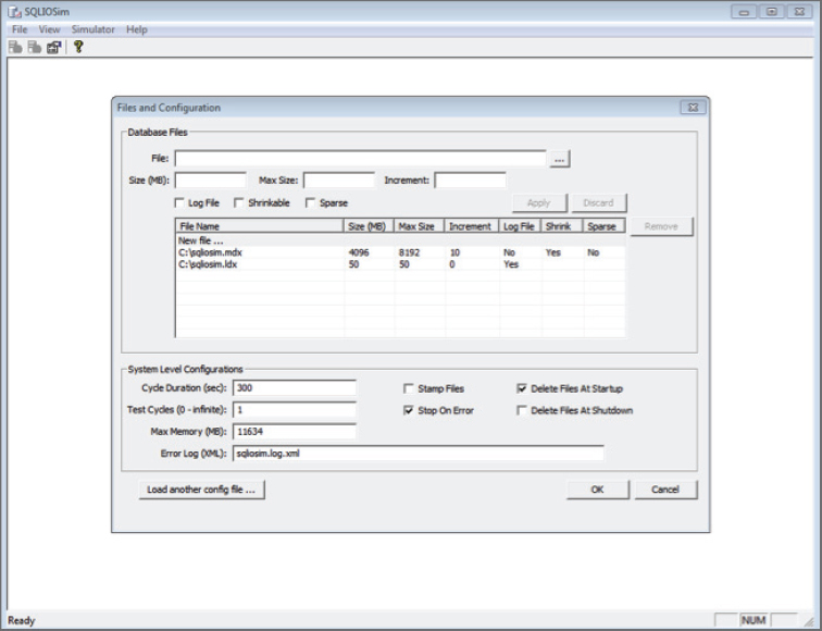
Before getting started, note that SQLIOSim will report an error if latency exceeds 15 seconds. It is perfectly normal for storage I/O to show occasional high latency. We recommend using the GUI to run functional system testing (Figure 4-13), although the tool can be also be executed from a command prompt.

SQLIO is a tool that simply generates I/O. This application is executed from the command line and does not need SQL Server to run. Download SQLIO from http://www.microsoft.com/download/en/details.aspx?displaylang=en&id=20163.

We recommend testing the storage system to performance maximums and setting up a test that mimics your best guess at a production workload. SQLIO is executed from the Windows command line. After installing SQLIO, open the param.txt file located in the installation directory. The default path is C:Program Files (x86)SQLIO. The param.txt file contains the following code:

c:	estfile.dat 2 0x0 100
#d:	estfile.dat 2 0x0 100

The first line in the param file defines where the test file is located. Use the pound sign (#) to comment out a line in the param.txt file. The first number following the test file defines the number of threads per test file. Microsoft recommends setting this to the number of CPU cores running on the host machine. Leave the mask set at 0x0. Finally, the size of the test file in MB is defined.

Ensure that the test file is large enough to exceed the amount of cache dedicated to your storage volumes. If the host file is too small it will eventually be stored within the array cache.

SQLIO is designed to run a specific workload per instance. Each time you execute SQLIO.exe with parameters, it will define a specific type of I/O. It is entirely permissible to run many instances of SQLIO in parallel against the same test file.

Be sure to coordinate testing with your storage administrator before you start these tests, as they are designed to heavily stress your I/O system. It is best to begin by confirming any calculated assumptions. If you have 100 10K SAS disks configured in a RAID 1+0 set, you can assume random I/O will perform 14,000 reads. To test these assumptions run a single SQLIO.exe instance:

sqlio –kR –s300 –frandom –o1 –b8 –LS –Fparam.txt

The –k option sets either R (read) or W (write). Set the test run length using the –s function. We recommend testing for at least a few minutes (this example uses 5 minutes). Running a test for too short a time may not accurately demonstrate how a large RAID controller cache will behave. It is also important to pause in between similar tests. Otherwise, the array cache will reuse existing data, possibly skewing your results.

The –f option sets the type of I/O to run, either random or sequential. The –o parameter defines the number of outstanding I/O requests. You use the –b setting to define the size of the I/O request, in KB. This example tests very small I/O. SQL Server normally reads at least a full 64KB extent.

You use the –LS setting to collect system latency information. On a 64-bit system you can add the –64 option to enable full use of the 64-bit memory system. Finally, you define the location for the param.txt file using the –F option. Following is the test output:

sqlio v1.5.SG
using system counter for latency timings, 14318180 counts per second
parameter file used: param.txt
        file c:	estfile.dat with 2 threads (0-1) using mask 0x0 (0)
2 threads reading for 300 secs from file c:	estfile.dat
        using 8KB random IOs
        enabling multiple I/Os per thread with 8 outstanding
size of file c:	estfile.dat needs to be: 104857600 bytes
current file size:      0 bytes
need to expand by:      104857600 bytes
expanding c:	estfile.dat ... done.
using specified size: 100 MB for file: c:	estfile.dat
initialization done
CUMULATIVE DATA:
throughput metrics:
IOs/sec: 13080.21
MBs/sec:   102.18
latency metrics:
Min_Latency(ms): 0
Avg_Latency(ms): 0
Max_Latency(ms): 114
histogram:
ms: 0 1  2 3 4 5  6  7  8  9 10 11 12 13 14 15 16 17 18 19 20 21 22 23 24+
%: 37 59 3 0 0 0  0  0  0  0  0  0  0  0  0  0  0  0  0  0  0  0  0  0  0

This single 8K random test started by creating the 100MB test file. In this case, the test was generated on a VM guest using a flash drive, so the results are not representative of what you might see in a real-world test. The test ran for five minutes with one outstanding I/O, and generated 13,080 IOPS and 102 MB/sec. It peaked at 114 milliseconds of latency but averaged under a millisecond for access.

This test is a perfect demonstration of how a system can fail to utilize its maximum potential performance. Only eight outstanding I/Os completed, which failed to push the I/O subsystem. To properly test a given system, it is a good idea to scale the workload dynamically to determine how it will perform under increasing loads. To accomplish this you can script SQLIO:

sqlio –kR –s300 –frandom –o1 –b8 –LS –Fparam.txt
sqlio –kR –s300 –frandom –o2 –b8 –LS –Fparam.txt
sqlio –kR –s300 –frandom –o4 –b8 –LS –Fparam.txt
sqlio –kR –s300 –frandom –o8 –b8 –LS –Fparam.txt
sqlio –kR –s300 –frandom –o1 –b16 –LS –Fparam.txt
sqlio –kR –s300 –frandom –o1 –b32 –LS –Fparam.txt
sqlio –kR –s300 –frandom –o1 –b64 –LS –Fparam.txt
sqlio –kR –s300 –frandom –o1 –b128 –LS –Fparam.txt
sqlio –kR –s300 –frandom –o1 –b256 –LS –Fparam.txt

Run this batch file from the command line and capture the results to an output file:

RunSQLIO.bat > Result.txt

Ideally, you will test several different scenarios. Create a batch file with each scenario that scales from 1 to 256 outstanding I/Os, such as the following:

• Small-block random read performance:

  sqlio –kR –s300 –frandom –o1 –b8 –LS –Fparam.txt

• Small-block random write performance:

  sqlio –kW –s300 –frandom –o1 –b8 –LS –Fparam.txt

• Large-block sequential read performance:

  sqlio –kR –s300 – fsequential –o1 –b8 –LS –Fparam.txt

• Large-block sequential write performance:

  sqlio –kR –s300 –fsequential –o1 –b8 –LS –Fparam.txt

Running these scenarios as a single batch file will automate the I/O system testing process. The most important data points are the latency and performance measurements. When the tests exceed your maximum latency tolerance, usually not more than 20 milliseconds, you have exceeded the capabilities of your I/O subsystem. If the system does not meet your overall performance requirements with adequate response times, then you need to investigate the system for errors or configuration issues. Ultimately, you may need to optimize the storage system’s performance to ensure that previously specified requirements are met.

SUMMARY

Database professionals can avoid I/O problems by designing, testing, and monitoring storage systems. You don’t need to be a dedicated storage professional to ensure reliable system performance; just follow these simple guidelines:

• Include I/O systems when designing and planning database systems.
• Always test the storage systems for functionality and performance.
• Continuously monitor storage performance. Establish lines of communication with storage administrators to ensure that the storage systems meet your requirements.
• Plan for recovery and/or disaster. Document your plan and test it to ensure that it can be executed.