C H A P T E R  5

Implementing Dashboard-Style Report Objects

Charts, maps, indicators and other Reporting Services objects add visual interest to reports. Many of these objects also allow you to communicate a great deal of information at a glance that would otherwise be time-consuming to discover from reading lines of detail in a report containing only columnar data. Reporting Services provides a number of chart types and other report objects that have their own purpose. The visual report objects at your disposal are:

• Chart: SSRS provides many chart styles that can be incorporated with other report objects such as the Table or Matrix or used as a stand-alone report.
• Gauge: Released with SSRS 2008, these visually appealing controls provide at-a-glance views, typically used as Key Performance Indicators of business measurables, such as sales and profit trending. Prior to SSRS 2008, gauges had to be acquired separately.
• Image: This report object can embed standard format images, such as JPEG or TIFF, directly in a report. You can embed images directly in reports, say for a company logo, or pull them directly from a database table.
• Map: The map object allows developers to add overlaying visualizations on top of aerial maps to represent data returned by a map gallery, a spatial query or from Environmental Systems Research Institute, Inc (ESRI) objects and shape files.
• Data Bar: This report item can be used as a horizontal bar or vertical data column. It is often used to convey a lot of information in a smaller amount of space than typical bar charts. For example, you might use a data bar if you wanted to visually represent the test scores that a group of students received on a particular assessment.
• Sparkline: Much like the Data Bar, this report object is usually used to visualize large amounts of trending data on a particular measure, but in a more condensed fashion than the traditional chart provides. This is much like the depiction of the price of stock over a given date range with few or no labels and legends present.
• Indicator: Added in SSRS 2008 R2, this report item can be used to show different images that visually represent a certain predefined or data driven value. Examples of this object are commonly seen in report sections that provide a comparison against a Key Performance Indicator (KPI).

The rest of this chapter takes you on a tour of SQL Server 2012 Reporting Service’s charting capabilities. First, we’ll cover some needed ground pertaining to the chart data region. Then we’ll work through some examples of the available charts.

Understanding the Chart Data Region

The Chart data region of SSRS, like the Matrix data region, allows multiple grouping levels from a single dataset. Instead of the column- and row-level groupings that the Tablix data regions provide via Table, Matrix, and List objects, the Chart data region uses Series, Categories, and Values. You can set many properties for a chart, and as with all other data regions, a chart can use expressions to define its properties. In addition, as with other data regions, you can place charts by themselves or scope them within another region such as a List or Table data region. For example, you could use a simple chart to show the overall visits by type of clinician, which in your stored procedure is determined by the Service_Type field. You could also add the chart to a cell in a table that’s grouped by patient and time frame, such as Month and Year. The chart would show for each grouping a visit count for that patient over time. Let’s add a chart to the report that uses the Emp_Svc_Cost stored procedure. For the chart, you will add three familiar fields, one for each chart area: Series, Categories, and Values will contain Patient_Name, Employee_Name, and Visit_Count, respectively.

The starting-point report for the Chart object demonstrated in this section is available in the Pro_SSRS project in the Source Code/Download area for the book on the Apress Web site (www.apress.com). This report is called, creatively enough, Chart Start.rdl, which is also a breakfast cereal for corporate executives.

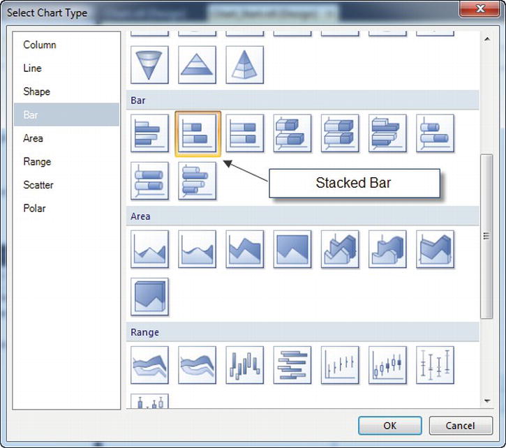
1. To begin, open the Chart Start.rdl report to the Design tab and double-click the Chart tool in the Toolbox to bring up the Select Chart Type dialog box. The Chart objects in SSRS 2008 were enhanced quite extensively, but mostly the updates are cosmetic. You will select the Stacked Bar chart shown in
   

   Figure 5-1. SSRS chart selections

2. Double click the graphic area of the chart, which will bring up the Chart Data window.
3. Under the Values area of the Chart Data window click the green plus sign and select Visit_Count from the drop down list.
4. Next, click the green plus sign in the Category Groups area of the Chart Data window and select Employee_Name.
5. Next, click the green plus button in the Series Group area of the Chart Data window and select Patient_Name
6. Finally, resize the chart by dragging the bottom right corner down and to the right so it resembles Figure 5-2.

Figure 5-2. Chart with three fields

Before you preview the chart, let’s look at its properties. You will want to change the default palette to Light for a more subtle and visually appealing view. Right click in the chart and select Chart Properties under the Chart submenu. Choose the color palette named Light and select OK. The properties should look like Figure 5-3.

Figure 5-3. Chart properties

Finally, right-click inside of the chart graphic area while on the Design tab, and select 3D Effects. Next, click the checkbox to enable 3D effects and click OK. Before previewing the chart, rename the title from Chart Title to Visit Count By Patient. You can now preview the chart, as displayed in Figure 5-4.

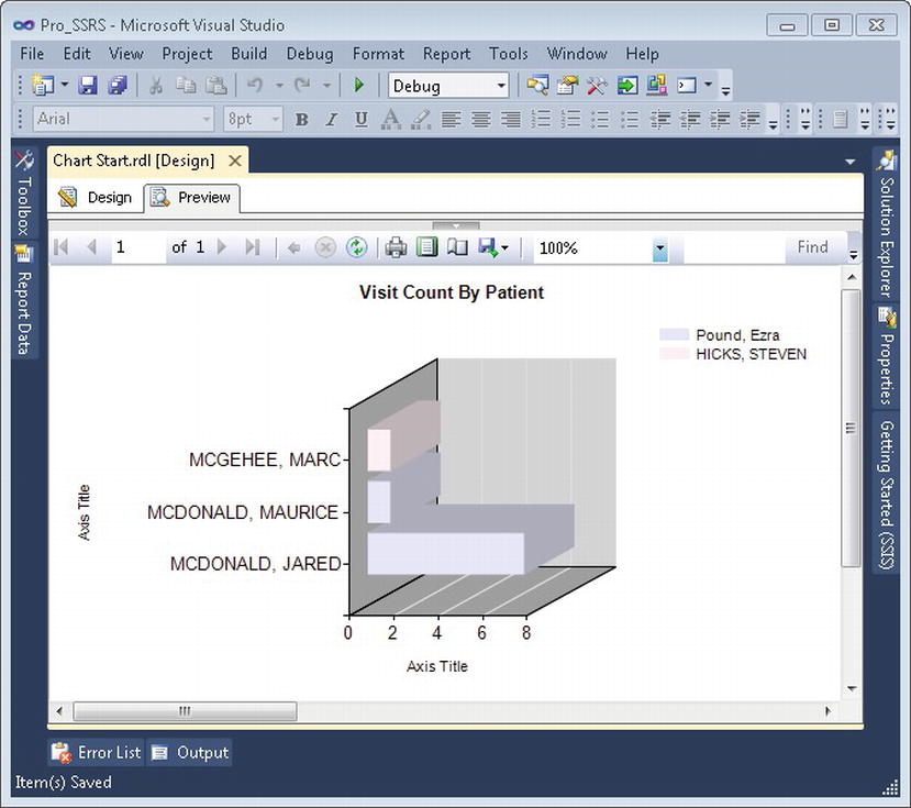
Figure 5-4. Chart with custom properties

You can see the RDL output for the chart you just created in Listing 5-1.

The completed report for the Chart object is in the Pro_SSRS project and is called Chart.rdl.

Implementing an Image

Having images in a report can give it a polished look while extending its value as a resource. Fortunately, SSRS includes an image tool that can add images from a variety of locations and supports many standard image formats. Our health care application stores many images in a SQL Server database as Binary Large Objects (BLOBs), as part of a patient electronic medical record (EMR). You can load any type of image into the database and associate it with the patient using a front-end image retrieval application. Once the image is in the database and tagged to a patient’s identification number, which is a field in the database, you can use SSRS to display that image in a report. For this sample, you will continue with the theme of famous author patients and add their images to a simple report. The starting-point report for the Image report object is called Image Start.rdl. Since much of the report is constructed using objects you have already used, the starting point is already laid out with these objects included. The dataset that is used for this report includes demographic information for patients who have their photographs stored in a database table called DocumentImage in the Pro_SSRS database. You can use the predefined dataset, called Get_Image, for the Image Start.rdl report, which simply returns patient demographic information for three patients along with their photos using a text query type as shown in Figure 5-5.

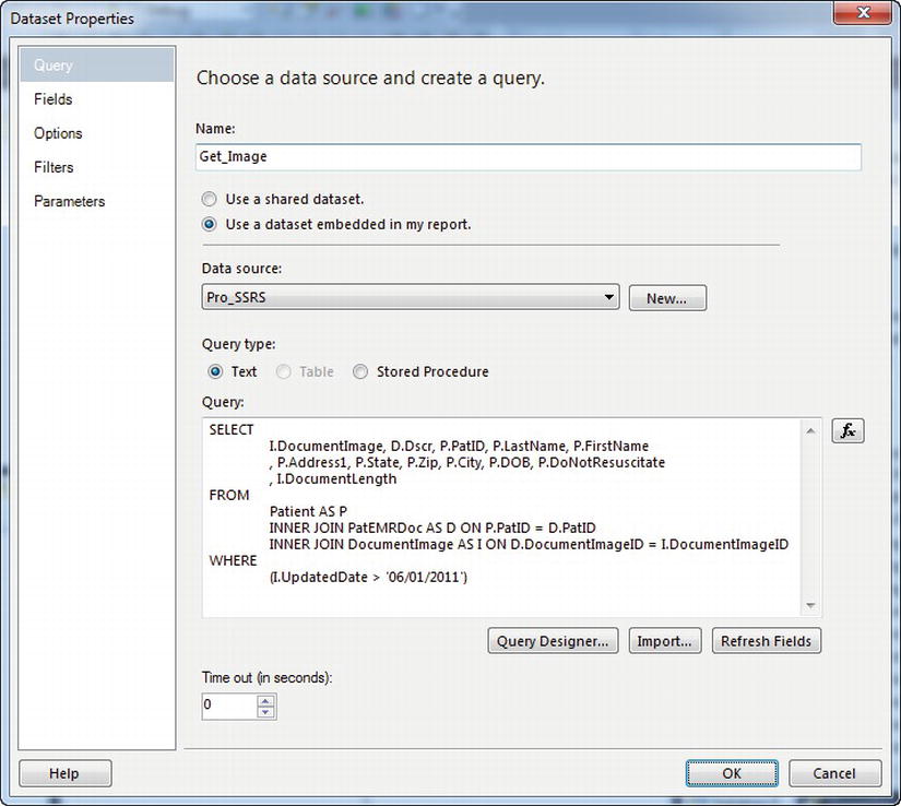
Figure 5-5. Get Image data set properties

Begin by opening the Image Start.rdl report in the Pro_SSRS project and clicking the Design tab. Next, select the Image tool from the Toolbox, and click into a blank area of the List data region that is already set up in this report. As you can see in Figure 5-6, you’re presented with the Image dialog when you add the Image tool to the list. You can choose several ways to retrieve images. For example, you could use an image that you’ve added to the project, or you could embed the image directly into the report. This option would serve you well if the report contained a single image that wouldn’t be used again and was intended to be distributed to a variety of sources that might not have access to the image at any other location. Choose Database for the source image. Next, you will choose the data source and field that contains the image. For this report, choose =Fields!DocumentImage.Value as the value, or as displayed, [DocumentImage]. Set the MIME type to image/jpeg.

The images stored in the DocumentImage field are patient photos. If this were a real report, you could use other images that would be standard to a patient record, such as X-ray images or photos of a patient’s wounds. Even scanned images of paper documentation or faxes could be stored in the database and effectively added to a full report.

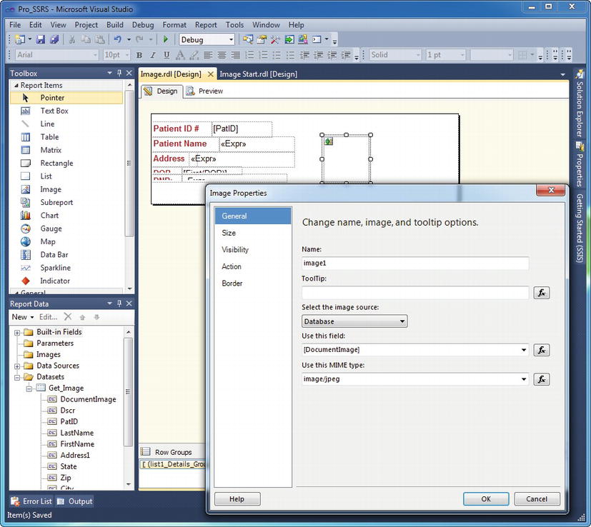
Figure 5-6. Image source selection

I would like to take a moment to point out a property that is not shown in Figure 5-6, but is very commonly used when using the Image object. Often times, the images need to be sized appropriately for the report being requested. For example, you may need to override the default of Fit Proportional to display an image in its original size or perhaps just a clip of it. Be careful when using the Fit to Size option, though, as this could cause your images to have a stretched appearance. You can set the sizing property in the Image Properties window on the Size tab or from the Properties window under Sizing as shown in Figure 5-7.

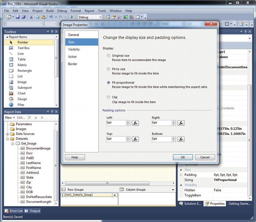
Figure 5-7. Image Properties – Appropriate sizing

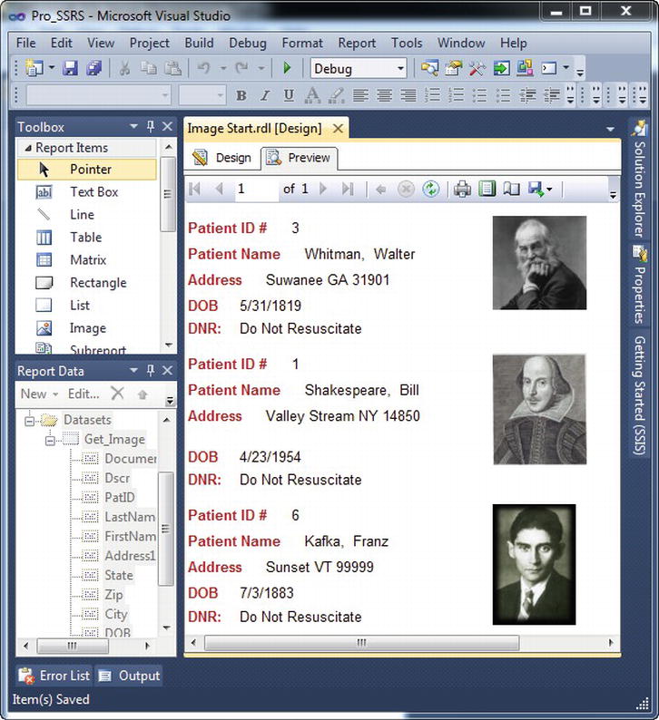
Figure 5-8. Preview of report with images

Listing 5-2 shows sample RDL elements for images.

The completed Image object report is called Images.rdl and is located in the Pro_SSRS project.

Implementing a Gauge

Gauges, although new in SSRS 2008, were available as a third-party add-in in SSRS 2005. However, such third-party add-ins had to be purchased separately. In SSRS 2008 and above, gauges are included by default and provide functionality that goes beyond standard charting. One nice thing about the gauge controls is that, while they add an aesthetic appeal to any report— a certain sexiness, if you will—they are also compact and provide an at-a-glance view of data that is so often important for business executives who only want to see highs and lows, ups and downs. With gauges, any value can have a threshold, and this threshold can be visually realized in the control itself.

Begin by opening the Gauge Start.rdl report included in the solution. Double-click the Gauge control in the Toolbox. The Select Gauge Type window will open displaying all of the available gauges. You have two types of gauges to choose from: Radial or Linear. As the names indicate, Radial gauges are round, like the speedometer in your car, and Linear gauges are straight, much like a standard thermometer. For this example, choose the 180 Degrees North gauge, as shown in Figure 5-9.

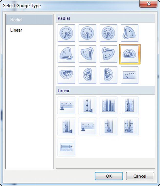
Figure 5-9. Radial gauge with range

We’ll walk you through creating a simple gauge range to show how the gauge pointer can be controlled by a value. On the Design tab, right-click the gauge and select Scale Properties under the Gauge Panel submenu. Change the Maximum value to 20,000 and click OK. Now, when you drag Visit_Count onto the data region of the gauge, the overall visit counts, which we know to be 9,687, will show as a range when the gauge is previewed (see Figure 5-10). We’ve only scratched the surface of the Gauge, but we will cover more detailed aspects of controlling the new gauge controls in Chapter 6.

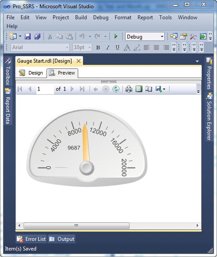
Figure 5-10. Radial gauge in preview mode

Listing 5-3 shows sample RDL elements for images.

Implementing a Map

Like the Gauge report item mentioned previously, a Map within a Reporting Services report was only possible through using custom or third party tools. In SQL Server 2008 R2, Maps were introduced to produce visually appealing reports that allow combining multiple layers over a topographical map. Each layer can get their data from a different dataset. Furthermore, you can integrate your map with Bing maps as easy as the click of a checkbox. The Map report item can consume data from a map gallery, an ESRI shapefile, or from a SQL Server spatial query.

A map gallery consists of RDL files created with coordinate and embedded vector polygons often created in tools like Mapwel, Map Maker Pro and ViLiDAR. There are some RDL files included in a standard installation containing the entire USA as well as each individual State. However, you can extend the maps that the wizard makes available to you as a report developer. As mentioned above, you can create your own vector polygons or even download those freely available on sites like CodePlex.com. Either way, in order for the Map Wizard to recognize them, you will need to save the RDL files in the path that the wizard reads. If you are using Visual Studio 2010 as I am, the path is Program FilesMicrosoft Visual Studio 10.0Common7IDEPrivateAssembliesMapGallery, under your Visual Studio installation directory. Some of the key elements in the RDL files are MapMeridians, MapParallels, MapLayers, and VectorData.

ESRI shapefiles store similar information about geographical, geometrical shapes, and informational data in files with .shp and .dbf extensions. When you select ESRI shapefile as your source of spatial data, you are prompted for a shapefile. After navigating to the shapefile, the geospatial data is embedded into the report. For an example of how an ESRI shapefile of Duval County in Jacksonville, FL looks, see Figure 5-11.

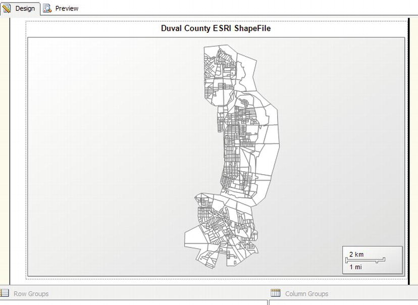
Figure 5-11. ESRI Shapefile of Duval County, Jacksonville, FL

The third way you can get your spatial data is by using a SQL Server Spatial query. This allows you to create your own queries to display geographical details along with quantifiable data. For example, it is easy to create a query that returns a listing of total sales amount for every State in the US. You can then overlay those details on top of a map.

We begin this example by opening up the Map Start.rdl report included in this section is available in the Pro_SSRS project in the Source Code/Download area for the book on the Apress Web site (www.apress.com). Double-click on the Map control in the Toolbox to start the Map Wizard. The first thing we need to do is let the map control know where we are going to get the spatial data from. We are going to use the map gallery (which is the default), so ensure that the radio button is selected, and then choose the USA by State Inset under the Map Gallery tree list, as shown in Figure 5-12. When you select a particular Map Gallery, you are shown a preview of your selection.

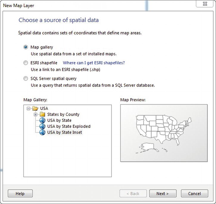
Figure 5-12. New Map Layer Wizard: Choose source of spatial data

Click on the Next button to go to proceed to Choose spatial data and map view options step of the wizard. On this screen, you have the option to set your zoom level, modify the resolution settings, and add in a Bing Maps layer. For now, let’s just keep the defaults on this and click Next to continue on to Choose map visualization as shown in Figure 5-13.

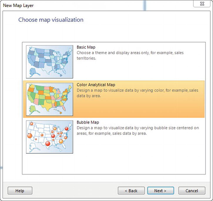
Figure 5-13. New Map Layer Wizard: Choose map visualization options

Select the middle visualization Color Analytical Map and click Next. On the Choose the analytical dataset screen, you need to select or create a dataset which includes the spatial data. You are going to use the existing dataset, so choose the Emp_Svc_Cost_By_Patient_State dataset and click Next to proceed. On the Specify the match fields for spatial and analytical data screen, you need to select which fields in your dataset match with Map Gallery that you selected. In this case, the wizard realized that you had a StateName field and automatically creates a link to it, as shown in Figure 5-14. If you didn’t have StateName but you had the state abbreviation, you would need to specify what field in your dataset would match. In that case, you could match your State column to the STUSPS spatial data column. Be sure that the Match Fields has the checkbox next to STATENAME and the Analytical Dataset Fields is set to StateName and click Next to proceed to the Choose color theme and data visualization screen.

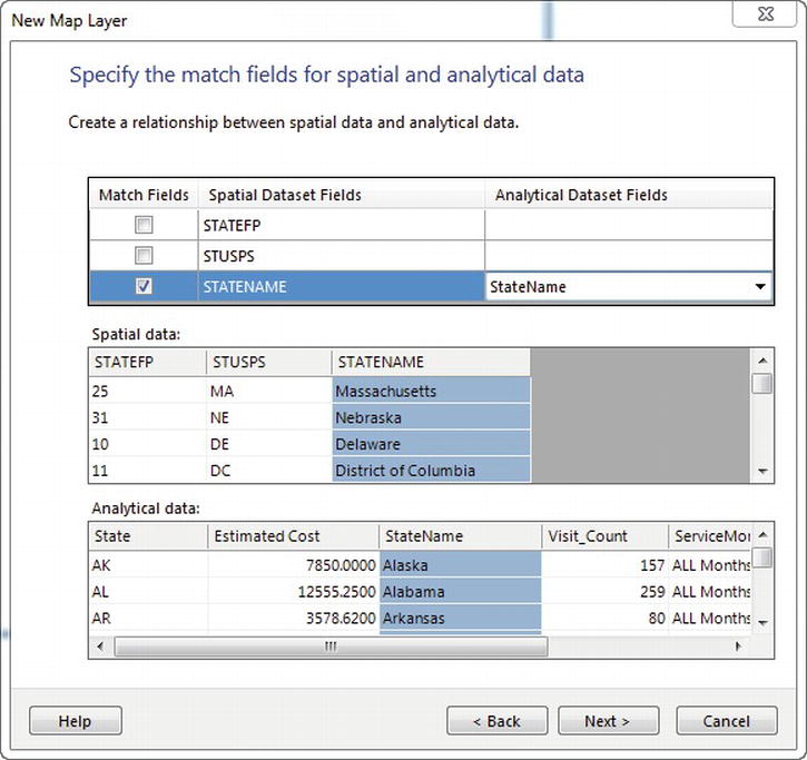
Figure 5-14. New Map Layer Wizard: Specifying fields to match on

Modify the Field to Visualize to use [SUM(Visit_Count)], enable the checkbox option to Display labels and set the Data Field to be used as [SUM(Visit_Count)] as well. Figure 5-15 shows the settings on the map’s final wizard screen.

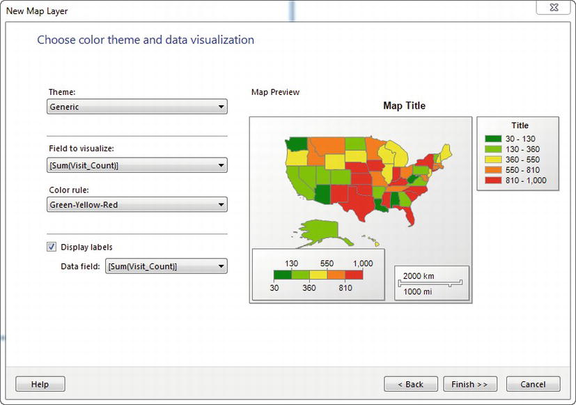
Figure 5-15. New Map Layer Wizard: Choosing color theme and visualization

Click Finish to complete the Map wizard and click the Preview tab as shown in Figure 5-16 to see the map in action.

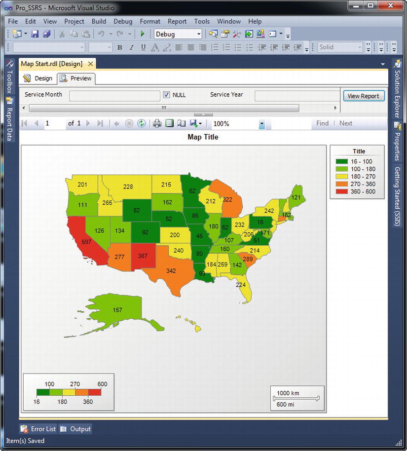
Figure 5-16. Map using spatial query

Listing 5-4 shows sample RDL elements for images.

The completed Map object report is called Map.rdl and is located in the Pro_SSRS project.

Implementing a Data Bar

Another new addition to Reporting Services 2008 R2 was the Data Bar. For those of you who are savvy Excel users, you may recognize this report object from your tinkering in Excel. This object is essentially a single bar chart (most often displayed horizontally) which allows for a quick at-a-glance, row by row comparison. Longer bars equate to higher values and shorter bars unequivocally mean lower values.

In this example, we are going to start with the report named Data Bar Start.rdl in our Pro_SSRS project. You will notice that there is a dataset named Emp_Svc_Cost_Data_Bar already defined that executes a stored procedure to return the top ten States and the amount of visits for the specified ServiceMonth parameter. We also have a table with only two columns. Expand the Emp_Svc_Cost_Data_Bar dataset and drag the StateName field into the first column of the details row in the table. Next drag the Data Bar report item into the second column of our details row. Upon releasing the Data Bar, you will be prompted to select the type of Data Bar that you want. Your options are:

• Bar
• Stacked Bar
• 100% Stacked Bar
• Column
• Stacked Column
• 100% Stacked Column

For this example, choose Bar as shown in Figure 5-17 and click OK.

Figure 5-17. Data Bar Type Selection

Next, drag the Visit_Count_By_State field over top of the Data Bar and hover over it until the Chart Data dialog box pops up. When you see the Chart Data dialog, drag the selected field into the white space of the Values section, as shown in Figure 5-18.

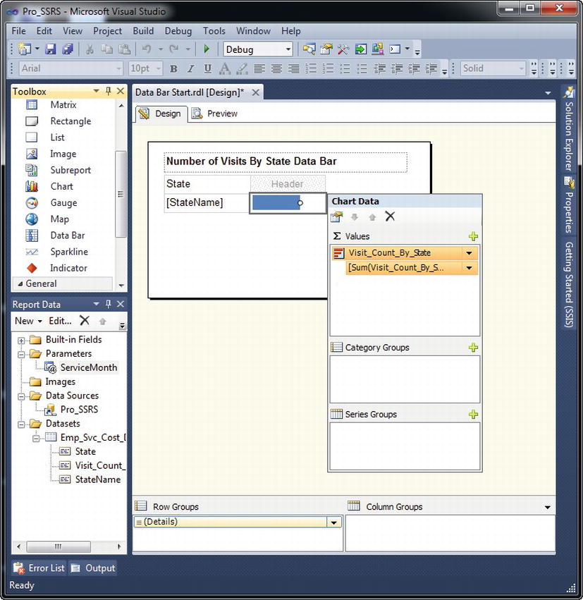
Figure 5-18. Data Bar: Chart Data Value

You could stop here, but let’s add a little more pizazz to the report. Label the header column with the Data Bar “Visit Count.” Then make the header row Bold and Centered. Now, select the Data Bar—the blue bar and not the cell—and then right click it to bring up the dialog box and choose Show Data Labels. This will show the values when you run the report. Next, right click the Data Bar again and then select Series Properties… Go to the Fill tab, select Gradient with a Gradient style of Left right, as shown in Figure 5-19. Then click on the f_x button next to the primary color (top color) to create an expression.

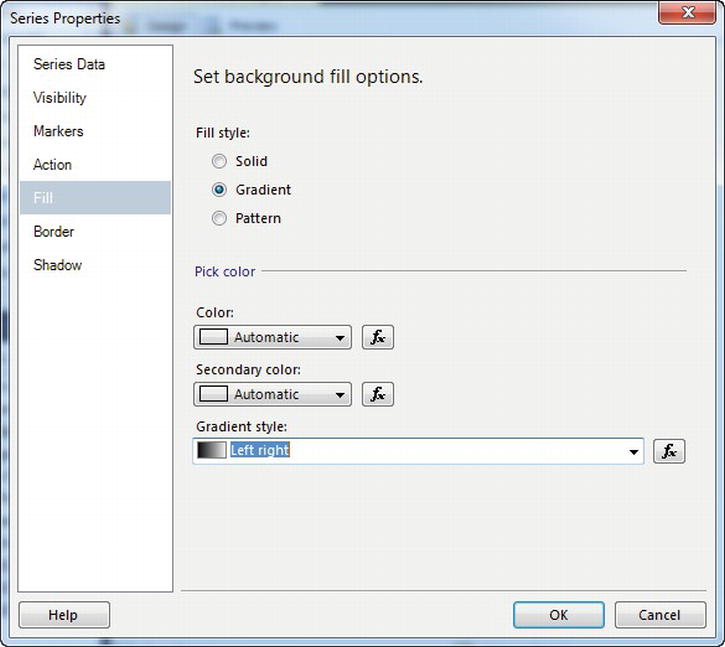
Figure 5-19. Data Bar: Series Properties fill options

Once you have the expression editor open, enter the following expression and click OK:

As shown in this expression, you can nest your conditional statements. Here we are checking to see if the parameter label selected was not ALL. Then it checks for the Visit_Count_By_State to see if it is more than 75 for the month selected. If it is, then make the Data Bar green and if not, make it red. The outer IIF statement checks to see if the count is greater than 300 and sets the colors accordingly. Click Preview to see your report in action, as shown in Figure 5-20.

Figure 5-20. Preview of the Data Bar Report

Listing 5-5 shows a section of the RDL file for the Data Bar report item.

The completed report for the Data Bar is called Data Bar.rdl in the Pro_SSRS solution.

Implementing a Sparkline

At least in my experiences, a common report request by leadership has been to show a month over month or year over year trend analysis. One could do this in prior versions of Reporting Services, but it took a little more effort to get the look and feel of a true trending report. Included with 2008 R2 release of Reporting Services was the Sparkline control. This out-of-the-box report item is simple to use and can display vast amounts of data in a small area.

In this example, we will start by opening the report named Sparkline Start.rdl in our Pro_SSRS Reporting Services solution. You will notice that we have created a dataset which executes a stored procedure named Emp_Svc_Cost_Sparkline. This stored procedure returns the Date, Month and Year a particular visit occurred. You’ll also find a Tablix containing the month field from our dataset and some appropriate headings.

To start this example off, drag the Sparkline control from the Toolbox and place it in the blank textbox below the Daily Trend header and choose the Area sparkline type. This is the first type under the Area section. The other three types could be Smooth Area, Stacked Area and 100% Stacked Area. Next, expand the Emp_Svc_Cost_Sparkline dataset and drag the Visit_Count field on top of the new Sparkline. If you hover over the Sparkline before releasing, you will see the Chart Data screen as you have seen in earlier examples. Release the Visit_Count field into the Values section, as shown in Figure 5-21.

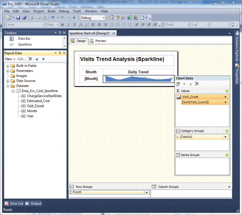
Figure 5-21. Sparkline: Chart data value

Upon previewing the report, you should see a daily trend of visits. It may seem a bit rough right now, but we’ll make it a little nicer in a minute. You’ll also notice a parameter for MonthlyGoal that we are about to implement as a variation of a key performance indicator or KPI. As we did in the Data Bar example, we are going to change the color of our Sparkline to be a shade of Red or Green, depending on whether we met our monthly goal of visits. Click the Design tab to make some more edits to our Sparkline report.

Double click on your Sparkline control and then right click Visit_Count in the Chart Data window. Choose Series Properties and navigate to the Fill tab. Select Gradient as the Fill Style, White as the Secondary Color and a Gradient Style of Top Bottom. Finally, let’s set an expression to change color based on our MonthlyGoal parameter. Click the f_x button to the right of the top color choice to create an expression. Clear out the default text, enter the following expression, and click OK to close the expression editor. The Series Properties window should appear as Figure 5-22.

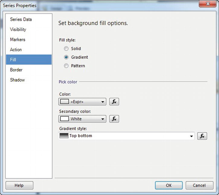
Figure 5-22. Sparkline: Series fill options

We’ll be covering expressions later, but this expression is essentially comparing the total count of visits for the month group against the value selected in the monthly goal parameter. Figure 5-23 displays the report in preview mode. Change your Monthly Goal to 2000 and click the View Report button to see the dynamic nature of our color expression. Normally, KPI’s are not implemented in this manner, but one could see how to use a value to dynamically change the colors to provide an at-a-glance visual indicator as to the success or failure of meeting predefined goals. Normally, these values would be stored in a database to allow the value to be configurable.

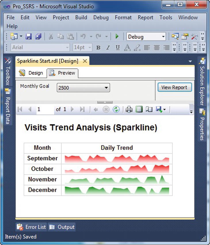
Figure 5-23. Sparkline: Previewing the report

Listing 5-6 shows a section of the RDL file for the Sparkline control.

The completed report for the Sparkline is called Sparkline.rdl in the Pro_SSRS solution.

Implementing an Indicator

In Reporting Services 2005 and 2008, we could create the functionality that we see in reports containing KPI’s. However, it took a little creativity in the use of expressions. For example, if you wanted to show an image based on a certain value in a result set, you would need to set the visibility of each of the images to be based on an expression. That approach is not too difficult to implement, but it is a more difficult to maintain. In 2008 R2, we were provided this functionality right out of the box with the Indicator report item.

Often times, the consumers of our reports like to see a visual indicator as to the trend in a basic directional fashion. For example, one may want to see if the total visits were higher than last month, the same or was it less. If we see a consistent trend of negative results, decision makers may want to dig deeper into the possible causes. This is the style of the report that we are going to create in this example. Our decision makers want to see the current state of total visits in relation to the prior month.

In this example, we will start off with Indicator Start.rdl in our Pro_SSRS solution. Included in the Indicator Start report is a dataset that returns four years of sample visit data. You will also notice that there is a tablix with three columns. Two of these already have some of the data needed on the report and a third will be used for our Indicator report item. We have shown you some of the ways to add items to your report design surface, but as with many applications, one can often complete the same task several different ways.

Right click on the empty textbox in Tablix1, select Insert at the bottom of the sub-context menu, and choose Indicator. When you add an Indicator report item to a report, you are prompted with the Indicator Wizard as shown in Figure 5-24. There are four categories of indicators which you can choose. However, each of these indicators can be customized down to the color and the values used to control them. You can even add more indicator states, use your very own custom images, or embed images within the Gauge control.

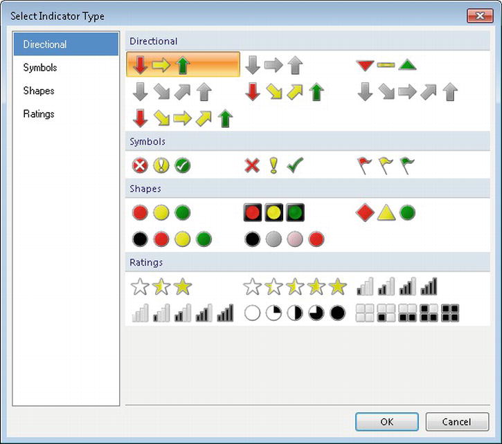
Figure 5-24. Indicator: Indicator type selection

We are going to use the default Directional indicator, the one with three arrows. Be sure that indicator is selected. Then click OK to return to the report designer. At this point, we have added an indicator, but we have yet to tell it what field to use. Right click on the indicator, select Indicator Properties and choose the Values and States tab. This is the screen where most of the magic happens. Set the Value to be =SUM(Fields!Diff.Value), as you want to display the difference between the current month and prior month as shown in Figure 5-25. Next, switch the States Measurement Unit to Numeric from Percentage. If your results were coming back as a percentage of change value, then you would leave this at its default setting. If you wanted to add or reduce the number of indicator states, you could do that by clicking the Add or Delete buttons, respectively. Three values will suit our needs in this example, so make the following changes to the start and end values:

• Red Down Arrow – Clear the start value and set -1 as the end. This essentially is telling SSRS that anything negative should be represented by the red down arrow.
• Yellow Right Arrow – Set the start and the end values to 0 to represent no change in the current and prior total visit counts.
• Green Up Arrow – Enter a 1 in the start value and clear out the end value to show all positive values as an increase in visits over prior month.

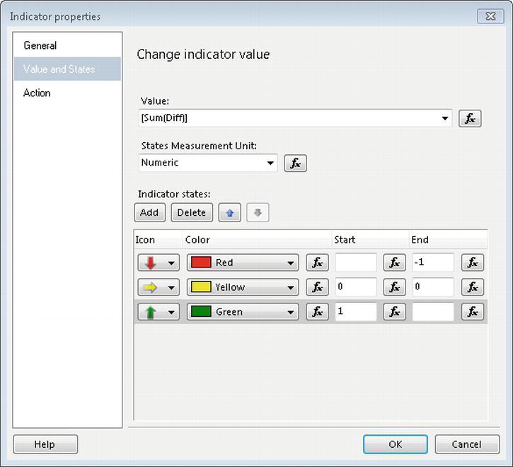
Figure 5-25. Indicator properties

After you have made the required changes, click OK to return to the Indicator Start report. Click the Preview tab to run the report. If all settings are set appropriately, your report should look like Figure 5-26.

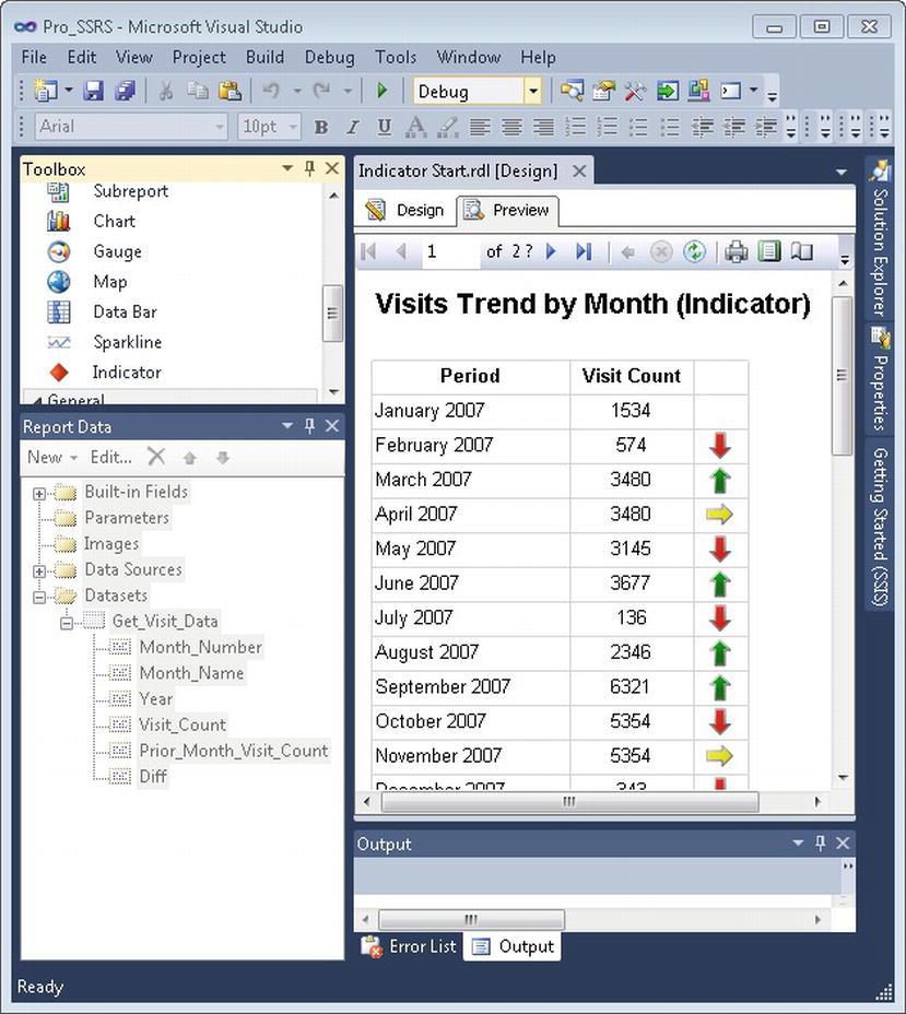
Figure 5-26. Preview Indicator Start

Listing 5-7 shows a consolidated section of the RDL file for the Indicator report item.

The completed report for the Indicator is called Indicator.rdl in the Pro_SSRS solution.

Summary

In this chapter, we covered some of the more visually appealing objects in Reporting Services, such as charting, maps, and gauges. Most of these objects are typically found in dashboard style reporting to provide an at-a-glance perspective. We also went over the chart data region and walked through examples of the different chart types available. Now that you’re more comfortable with the design environment, you’ll learn how to use it to design and deploy some real reports. In the next chapter, we’ll show how to take a step-by-step approach to adding these report items to a report that was designed as part of an SSRS migration for a health care application.