C H A P T E R  13

Creating Reports Using Report Builder 1.0, 2.0, and 3.0

When it comes to user-developed reports, we often have to deal with the problem of providing the underlying data in a controlled and secure way, but with enough freedom for that data to be useful for making business decisions. In SQL Server 2005, Reporting Services included the first version of the Report Builder. Report Builder is an application that offloads some of the tedious report design tasks to the report consumers themselves.

In Report Builder 1.0, users with appropriate permissions could create and publish their own reports with one caveat: the data had to be provided using a predesigned report model. This report model created an abstraction layer, if you will, that allowed the users to use the provided attributes as report elements. As with any new advances in software development, we often find some functionality is deprecated. In that regard, SQL Server 2012 is no different. We can no longer create Report models using the 2010 version of BIDS, SSDT, or Visual Studio, but we can still utilize them as a data source within our reports.

With the release of SQL Server 2008 came the Report Builder 2.0 application. With its Ribbon technology, akin to other Microsoft Office products, Report Builder 2.0 delivered a familiar interface and trumped Report Builder 1.0 by allowing users to write queries and use stored procedures to access data directly from the database, without the extra abstraction layer of a report model. This new interface was intuitively easier to use, with capabilities that far exceeded those of Report Builder 1.0.

In April of 2010 came the release of SQL Server 2008 R2 and with it came another version of the Report Builder that offered dataset caching and integration with the enhanced visualization report controls like the Map and Sparklines, as well as Indicators. Since you are now familiar with producing reports using BIDS, let’s turn our attention throughout this chapter to creating practical real world reports in Report Builder 1.0, 2.0 and 3.0 applications.

One thing to note before we get started is that, at the time of writing of this book, the vast majority of organizations are still using prior versions of SQL Server. As such, we decided to keep Report Models and Report Builder 1.0 in this version of the book. If SQL Server 2012 is the only version that your organization owns, or if your company is planning to migrate everything to SQL Server 2012, you can skip over the Report Model and Report Builder 1.0 sections. If your company is one of those migrating to 2012, just know that there is currently no path for migrating Report Models to SQL Server 2012. With that caveat behind us, let’s get started.

First, we will explore Report Builder 1.0 and its components. As you will see, even though the user who compiles the report needs to do some design work, the administrator still needs to design the report model that provides data to the Report Builder 1.0 client application. We will walk you through the process of using Report Builder 1.0 from two vantage points—developing and publishing a report model based on user input and then creating your own ad hoc reports based on that model. The three steps we will cover are gathering user feedback, creating and publishing the report model, and finally testing the report model by creating reports with Report Builder 1.0:

Getting feedback: Since we have worked alongside developers for many years, we know that one of the biggest problems with delivering a new application is that sometimes users get the application and expect it to do more than it does, or expect it to do something in a different way than delivered. The expectation from a user’s perspective is that the system should do exactly what the user needs. But for a developer, if it doesn’t do it in version 1, it will have to do it in version 2. You can avoid this conflict by implementing standard design practices, which always take user feedback into consideration up front. This process is especially important when the same application will be delivered to different companies with users from different backgrounds, each with their own interpretations of how a process should work. In the past few decades, a system analyst would take information from groups of users and translate this to a technical design that the developer could slowly digest. Today, most system analysis work is done directly by the developer, who interacts with users during the design phase of the project. Before we cover how to build a report model to be used by report designers, we will provide a sampling of some of the feedback we have received about the kinds of reports users would like to see.

Building the report model: The report model is the heart of Report Builder 1.0. Report models serve as semantic descriptions of the underlying data source. Because the report model can simplify a potentially complex overall database schema by selecting individual tables, fields, and values, it can be likened to a SQL Server view. Indeed, a key component of the report model, as you will see in this chapter, is a data source view. Once DBAs or developers have created a report model that contains the data to meet the requirements of the users, they can publish it to the report server where it can be used by Report Builder 1.0, which is the client-side report designer. All the data provided to Report Builder 1.0 come from published report models. We will show how to create and publish models in this chapter based on user feedback.

Using Report Builder 1.0: Report Builder 1.0 is one of several design applications that can be used to create and publish SSRS reports without requiring a full development environment like Visual Studio or BIDS. Report Builder 1.0 relies on pre-published report models as its data sources. As you will see, the interface for Report Builder 1.0 is intuitive; in fact, it is ideal for users who need to quickly create reports based on predefined report templates. Report Builder 1.0 not only allows users to design reports, but also serves as the publishing tool to deploy the completed report directly to the report server.

When we begin talking about Report Builder 2.0, where users have more control of the data they are accessing, you’ll see that much of the same concepts that you learned with respect to Report Builder 1.0 still apply. Developers may find themselves still creating views and stored procedures based on feedback from a user who will ultimately be designing the reports. Likewise, many developers may decide that Report Builder 2.0 has all of the features they need and will select it as their preferred development environment.

Getting User Feedback

At this point in the book, you have built a report, Employee Service Cost, which breaks down the cost of health-care visits at several levels. You designed this report using BIDS, and it contains several grouping levels, interactive sorting, and drill-down functionality. The dataset for this report is a stored procedure that provides the desired fields from several tables in the Pro_SSRS database. Like the reports you will build with Report Builder 1.0, this stored procedure and report were created based on feedback from users who needed it. One objective when creating the stored procedure was to design it not only to address the requirements for one report, but also to be versatile enough to be reused for other similar reports. We will cover this issue when we show how to build a report model to meet the needs of the users and the report designers who will be creating and publishing the reports with Report Builder 1.0.

In the health-care industry (namely, in post-acute care such as home health and hospice), you have to follow many reporting requirements for state and federal agencies. From cost reports to patient admission and discharge information, different reports are needed by different departments for different reasons. One group of reports that is used by every department is the patient census. This report shows all the patients who are currently admitted to the health-care facility and who are receiving services. The report can be as simple as an alphabetized listing of patient names or as detailed as all the demographic information about each patient, such as where they live and who to contact in case of an emergency.

Since the patient census is the most frequently requested report for customization, we will use it as the example in this chapter for the report model, making sure we provide enough data to meet both current and future needs.

For the patient census report example, imagine that users have requested to see a daily total of patients who have been admitted to the facility. Such patients all have common data associated with them that is important when looking at a census. The information answers these types of questions:

• What is the patient’s primary diagnosis?
• What branch office is the patient currently admitted to?
• What is the patient’s length of stay in the facility?
• How many active patients are in each branch currently?
• What is the patient’s address, phone number, and other key demographic information? (This type of census report, often referred to as a face sheet, shows a lot of information about a patient in a compact location.)
• If the patient was discharged, when did that occur and what was the reason? Is it because they recovered, or did they transfer to a hospital?

You can answer all of these questions and more with a single query, which can form the foundation of the report model. So, in the Pro_SSRS_2008R2 database, you will join several tables into a single data source view to provide the information needed to deliver the patient census. You have used most of these tables already when developing other reports, but we will review the database schema of the associated tables before showing how to build the report model. These are the tables you will use in this chapter’s example:

• Admissions
• Branch
• Diag
• Discipline
• Documentlmage
• PatEMRDoc
• Employee
• PatDiag
• Dischg
• Patient

Each table contains specific information that is relevant to the individual patient’s admission history, and together they will provide enough data to create many kinds of census reports for many departments within the health-care agencies. You know the kinds of questions you will need to answer, and the tables have been designed to deliver that information based on direct feedback and requests for users. Now, let’s move on to designing the query and building the report model.

Introducing the Report Model

Just because you don’t understand the intricacies of putting all the parts of a car engine together does not mean you can’t drive, right? The same can be said for report designers who will design and publish reports using the ad hoc Report Builder 1.0. In this case, you have little need to understand the pieces and parts of the database structure in order to build reports. It is unavoidable, though, that someone must understand the database schema, just as mechanics must understand brake pads and fan belts. Building a versatile report model, which the report designer will use to create reports, will most likely fall under the authority of the DBA, data analyst, or SQL developer, who will have an intimate understanding of the data sources. In this section, we will show how to use the feedback gathered from the report consumers to develop a report model for the patient census reports that will serve to make the data easily accessible with logical and intuitive field names.

You will perform the following procedures to create the report model for the Patient Census report model:

1. Create a report model project using BIDS/SSDT.
2. Create a data source.
3. Create a data source view.
4. Create the Patient Census report model based on the data source view
5. Publish the Patient Census report model to the SSRS server.

The process of building a report model consists of many individual steps, many of which are controlled entirely by stepping through available wizards. A report model can be complex or simple, based on your individual needs. For the sake of brevity, we will keep the sample model as simple as possible; you will be able to answer the feedback questions for the patient census, and you will be able to create and publish your own report model without any issues.

Create a Report Model using BIDS 2008 R2

In this section, you will create a report model project using BIDS 2008 R2. A completed version of this project is included in the Source Code/Download area for the book on the Apress Web site (www.apress.com). When you open the solution, you will notice an already created report model called Patient Census Book. If you would like to publish the Patient Census Book report model as it is in the project to your SSRS server and begin working with the client-side Report Builder 1.0 application, just be sure to set the data source settings and deploy appropriately. In that case, just skip to the “Creating Reports with Report Builder 1.0” section. To follow the steps to create each piece of a report model using Business Intelligence Development Studio for SQL Server 2008 R2, from adding data sources and data source views to publishing the completed model, read on.

Open up BIDS on a machine that has BIDS installed for a SQL Server 2008 R2 installation. You will find BIDS by clicking on the Windows Start button, All Programs, SQL Server 2008 R2, and then SQL Server Business Intelligence Development Studio. Once BIDS is started, click on Project… next to the “Create:” label. As you can see in Figure 13-1, you can use several available project templates. Choose the Report Model Project template, name it Patient Census, add the appropriate location (in this case C:Pro_SSRS Project_2008R2), and click OK.

Figure 13-1. Creating a new report model project

A report model project has three main components: data sources, data source views, and report models, each one relying on the previous one. In other words, a data source view requires a data source, just as a report model requires a data source view. If you have successfully created the Patient Census report model project, you will see these three components, as shown in Figure 13-2.

Figure 13-2. Viewing the new Patient Census report model

Adding a Data Source

Logically, the first step is to create a data source. Before we can create a data source connecting to our SQL Server 2008 R2 machine, you will need to restore the Pro_SSRS_2008R2 database, as described in the ReadMe.txt file available in the Source Code/Download area for the book on the Apress Web site (www.apress.com). After you have the Pro_SSRS_2008R2 database set up, we need to create a data source for our model. Right-click the Data Sources folder in the Solution Explorer and select New Data Source under the Add menu. This brings up the Data Source Wizard to create a data source for a report model. Figure 13-3 shows the first page of the Data Source Wizard. Fortunately, you can select to not display the first page every time you open the wizard by checking Don’t Show This Page Again.

Figure 13-3. Using the Data Source Wizard

You have two options when creating a data source through the wizard, as shown in Figure 13-4. You can either create a new one based on an existing or a new connection, or you can create a data source based on another object such as a data source already defined in another project. For this example, choose to create a new data source based on a new connection, and click New to open the Connection Manager.

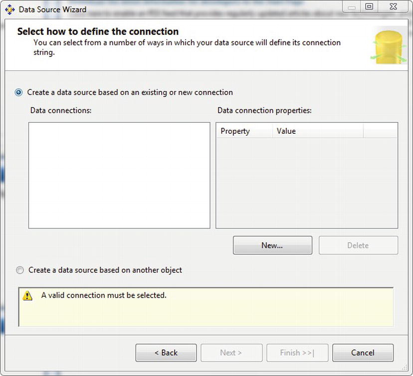
Figure 13-4. Defining a connection

In the Connection Manager, select localhost as the server name, leave the Use Windows Authentication button checked, and change the database name to Pro_SSRS_2008R2, as shown in Figure 13-5. Click OK to save the settings and return to the Data Source Wizard. Click Next or Finish to proceed to the final screen of the wizard, leave the default data source name of Pro SSRS 2008R2, and click Finish to create the data source.

Figure 13-5. Setting the server name and database

Creating a Data Source View

You create data source views for a report model project from relational data sources, where you have a list of tables that can be joined to form the basis of the data source view. In the Pro_SSRS_2008R2 database, you know many related tables are joined by column ID fields; for example, the Admissions table joins to the Patient table via the PatID field. Fields in both tables may be relevant to a user designing a report; however, superfluous data may just confuse that user. Part of your job as the report modeler is to remove the complexity of the schema but also provide a model that contains intuitive or “friendly” names and provides only the data that will be useful. Why should you use Dscr for a diagnosis code, when you really should just make it Diagnosis Name, for example? Since it is also possible to add objects to a data source view that are derived tables made from custom queries, you will have more control over creating a custom data source view and eliminate much of the work of removing the extraneous fields included in all the tables you are using. This will become more evident to you as you step through the process. For now, we will show how to perform the following logical steps to keep the data source view and subsequent model simple but effective:

• Building a query instead of many multiple tables for the data source view
• Selecting only relevant and potentially useful fields for the report designers, based on their requests
• Using friendly names for data source view fields and values

The first step in creating the view, like with the data source, is to open the wizard by right-clicking the Data Source Views folder and selecting Add New Data Source. Clicking Next to proceed to the next screen in the wizard will bring you to a screen depicted in Figure 13-6.

Figure 13-6. Adding a data source view to the project

On the first page of the wizard (not the welcome page, on which you should immediately check Don’t Show This Page Again), select the Pro_SSRS_2008R2 data source you created earlier, and then click Next to move to the Select Tables and Views page. As you can see in Figure 13-7, you can choose from many tables.

Figure 13-7. Related tables in the Pro_SSRS_2008R2 data source

You could add all the tables from the list of required tables for the patient census reports you are going to create; however, knowing that you will have too many unnecessary fields to work with, simply select Next and then Finish to close the wizard without including any objects. This will create the Pro SSRS 2008R2 data source view with no tables defined. Why, you may ask, did you not select any relational objects, since this seems like a crazy way to start? The reason is that you will add your own single object, called a named query, which is like a view in a SQL Server database. It is an object derived from a query of other objects. Assuming you had chosen one or more tables, you would have graphically defined the relationships for the tables based on primary keys, if they existed, or by using related column ID values and these tables would become the source for the report model. The end result is the same, whether you use real table objects with relationships or you use named query tables that contain only the fields you want. The difference is that this way you gain the benefit of one simple and concise table, instead of using many tables with the potential downside of adding more data than are needed for the model.

Once you have created the data source view, which defaults to a name of Pro SSRS 2008R2 based on the data source, you can double-click to open it in the design environment. It will appear empty, as it should. You can add the source query, or more accurately, the named query, by clicking the New Named Query button on the toolbar, as shown in Figure 13-8.

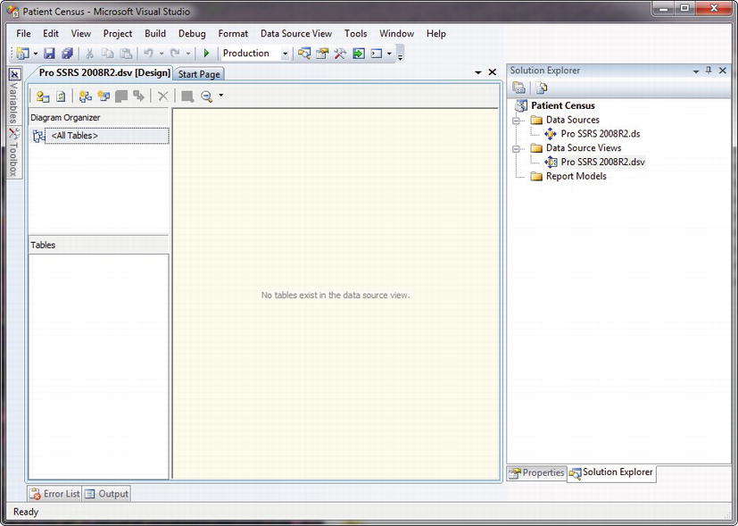
Figure 13-8. Pro SSRS data source view

In this case, you have already designed the query; however, Report Builder 1.0 includes its own graphical query builder, so it is possible to develop the query on the fly, so to speak. The graphical query designer is standard, with standard diagram, grid, SQL, and result panes. Clicking the New Named Query button opens the Create Named Query window. In the SQL pane, we can paste the pre-existing Patient Census query from Listing 13-1, and click in the blank diagram pane to automatically load the graphical representation of the query. If you need to provide aliases for any fields, such as distinguishing the common LastName fields from the employee and patient table, you can do that in the grid pane, as shown in Figure 13-9, which also shows the query and all the joined tables. Alias the lastname field as Pat_LastName for patient and Emp_LastName for employee. Otherwise, if there were common references to lastname, the default alias would have been ExprX, where X is the number of common references. You can do the same for the ubiquitous DSCR, used for descriptions, as in the Diag and PatEMR tables. We have also created an alias for each of the tables. This cuts down on the typing and makes the SQL easier to follow. You can alias the table names in the SQL section of the code or by Right-Clicking in the header section of each table and selecting Properties. You can enter the alias in the Alias section of the properties window.

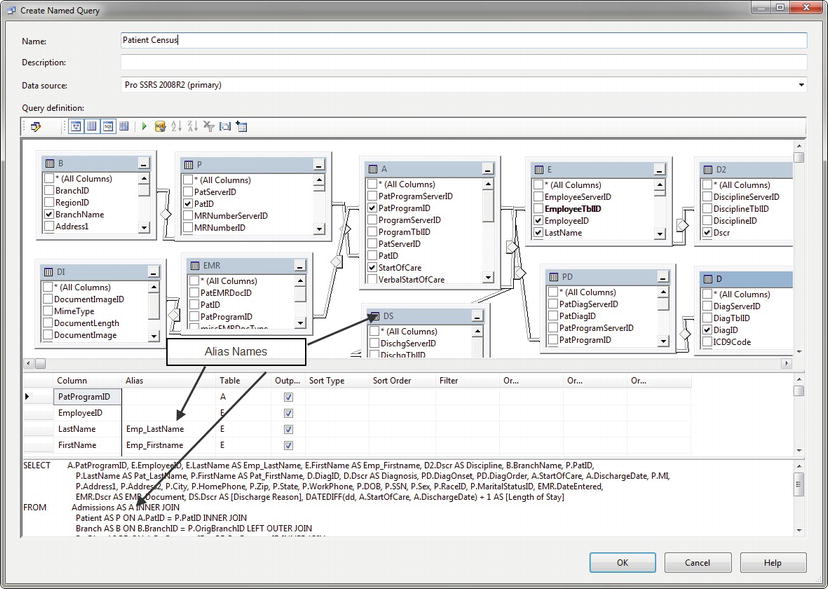
Figure 13-9. Named query displayed graphically with alias names

Finally, name the query Patient Census. When you click OK to complete the named query, your simple data source view consists of one object, Patient Census that contains the desired fields for the model. You can see in Figure 13-10 that 32 fields will be supplied to the model.

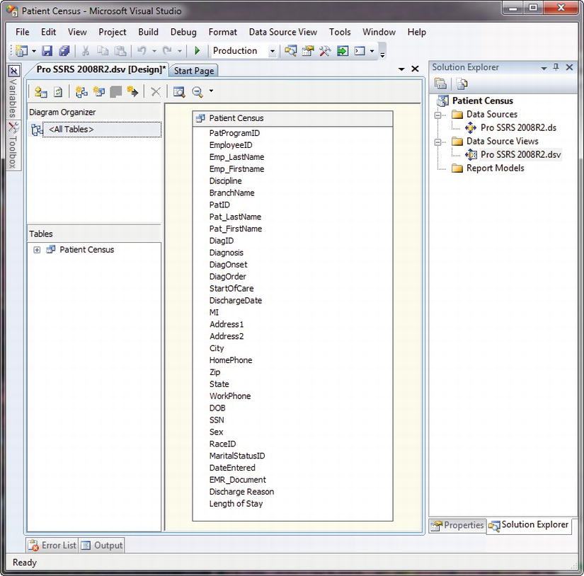
Figure 13-10. Data source view with one object

The next step in the process is to add a logical primary key to the Patient Census named query because the report modeler requires a primary key when it generates the model. Because the query is driven from the Admissions table, which contains the PatProgramID field that you know will contain unique values, you can use this field as the logical primary key for the Patient Census query. The PatProgramID field, in the example database, controls the admission and discharge records for a patient over time. It is typical that the same patient will be admitted to two separate service lines, referred to as programs; hence, you have PatProgramID. Without the PatProgramID field, the records would not be unique with the patient’s identification number, PatID, alone.

To set the logical primary key for the Patient Census object to be PatProgramID, simply right-click the PatProgramID field either in the Tables list or in the Patient Census diagram, and select Set Logical Primary Key, as shown in Figure 13-11. When you do this, you will see an icon that looks like a key appear next to the PatProgramID field.

Figure 13-11. Setting the logical primary key

At this point, you can save the data source view and then create the report model. Before you do, however, let’s take a look at a really great feature in the design environment, which is the ability to explore the data. Right-click anywhere in the Patient Census object—on EmployeeID, for example—and select Explore Data. As you can see, many records are returned from the entire Patient Census object, which you will use for the report you create later. However, also notice the three additional tabs beside Table, as shown in Figure 13-12. The Pivot Table, Chart, and Pivot Chart tabs suddenly appear, like finding a really valuable trumpet shell unexpectedly on the beach. (Not that this will help you greatly when developing the report model, but we just thought it was worth showing.)

Now that you have determined that the Patient Census data source view is returning data as you expected, you will save it and move on to the real heart of Report Builder 1.0, the report model.

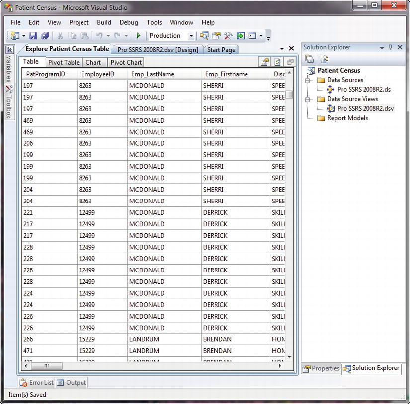
Figure 13-12. Additional tabs when exploring data

Creating a Report Model

The report model will add a layer of separation between report designers and the underlying data source, simplifying the process of designing reports by allowing them to focus on report design and not query design. Now that you have the data source view, which is a requirement for building a report model, you will learn how to create the model. The process is straightforward, thanks to auto-generation methods that analyze the data source view in two passes and produce the end result—a publishable report model in which the constituent elements would have otherwise taken much time and effort to produce, as you will see. The goal in this section is to walk you through the wizard so you can pay attention to the generation methods and finally deploy your completed model to the SSRS server.

You will again utilize the right-click procedure to initiate the Report Model Wizard from the Report Models folder in the Solution Explorer. After navigating past the first welcome page to the Select Data Source View page, you are presented with the Pro SSRS 2008R2 data source view selection, as shown in Figure 13-13.

Figure 13-13. Selecting a data source view

After selecting Pro SSRS, click Next, where you can now select the report model generation rules. You will see a set of rules that will be performed on the data source view. Several rules exist, and most of them are selected by default. Many of the rules are self-explanatory; however, two are not selected, by default: Create Entities for Nonempty Tables and Create Attributes for Nonempty Columns. These two rules instruct the generation process to create entities and attributes only for tables that contain data. Entities are the report model’s table equivalent, and attributes are conceptually the fields or columns defined within the entities.

The following are all the rules for the first pass of generating the model and are selectable in the Report Model Wizard:

• Create Entities for All Tables
• Create Entities for Non-empty Tables
• Create Count Aggregates
• Create Attributes
• Create Attributes for Non-empty Columns
• Create Attributes for Auto-increment Columns
• Create Date Variations
• Create Numeric Aggregates
• Create Date Aggregates
• Create Time Aggregates
• Create Roles

This pass processes all rules up to Create Roles. You will also see a helpful description for each rule, as shown in Figure 13-14.

Figure 13-14. Model generation rules with descriptions

For this example, leave the default selections, as these will give you features such as automatic aggregations for any numbers and dates and also create date variations so that for every Date Time data type in the data source view, you will have Day, Month, and Year created. You can click Next and choose to update statistics before generating, as shown in Figure 13-15. This is important if any data have changed significantly in the source tables.

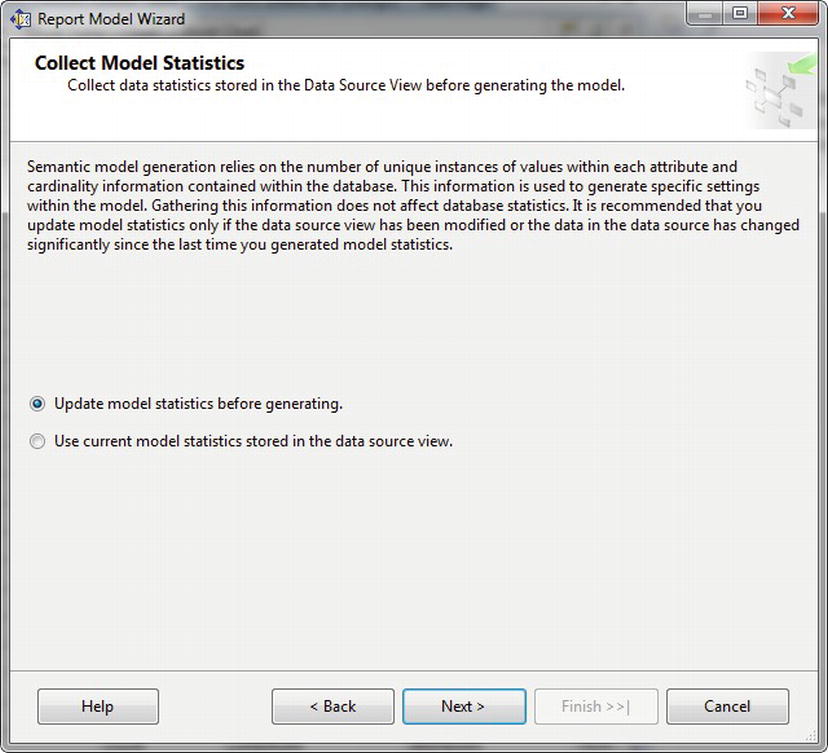
Figure 13-15. Update Statistics page

On the next page in the wizard, name your model Patient Census and select Run to begin the rules to generate the model. Figure 13-16 shows the output after clicking Run, and the process has completed successfully. You can see the details at each rule level of exactly what the rule did based on the data in the data source view. Notice that for Create Date Variations, for example, the rule discovered and created dates for DiagOnset, which is the date on which the patient was diagnosed with a disease. Other attributes that were created were Sum, Avg, Min, and Max for the Length of Stay column. The length of stay, usually an average, is the amount of time between the patient being admitted and being discharged from a long-term health-care facility. The DateDiff function calculates the length of stay.

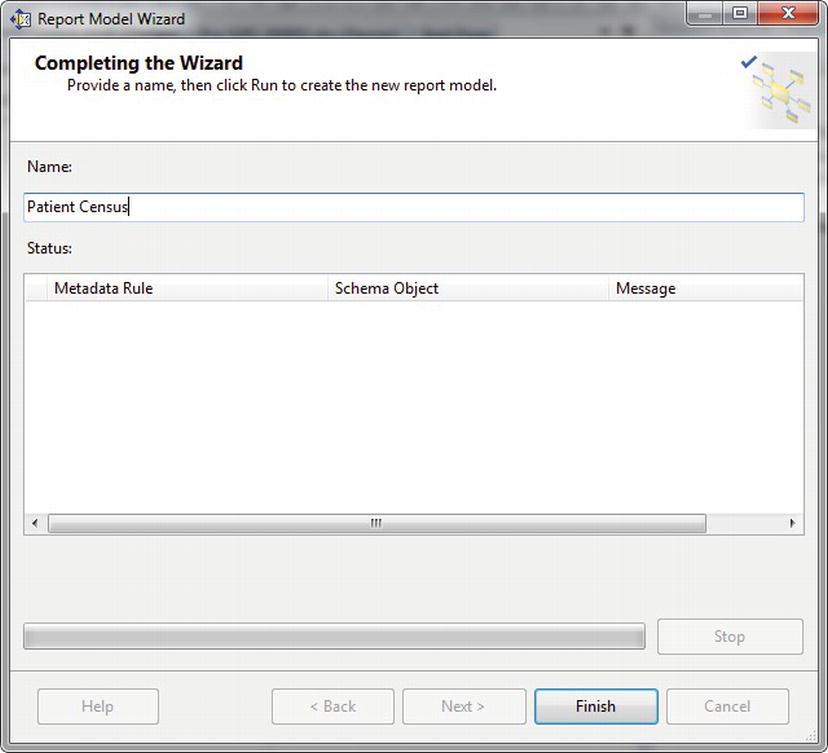
Figure 13-16. Rules completed successfully

After you click Finish in the Report Model Wizard, you can see that the Patient Census model has been created with the expected attributes. At this point, you can deploy the model directly to the report server by right-clicking the model in the Solution Explorer and selecting Deploy. You can control where the model will be deployed in the project’s properties pages, as shown in Figure 13-17, by clicking Project Properties under the Project on the toolbar. In this case, the project will be deployed to the Models folder on the report server, which has a target server URL of http://localhost/ReportServer. The data sources for the model will be published in the Data Sources folder.

Figure 13-17. Project properties for the report model

After you deploy the model, you can see in Report Manager the two folders that were created, Data Sources and Models. The Data Sources folder contains the Pro_SSRS_2008R2 data source, and the Models folder houses the Patient Census report model. Figure 13-18 shows the properties of the Patient Census report model. Just as with a standard data source, it is possible to view which reports have been created using the model.

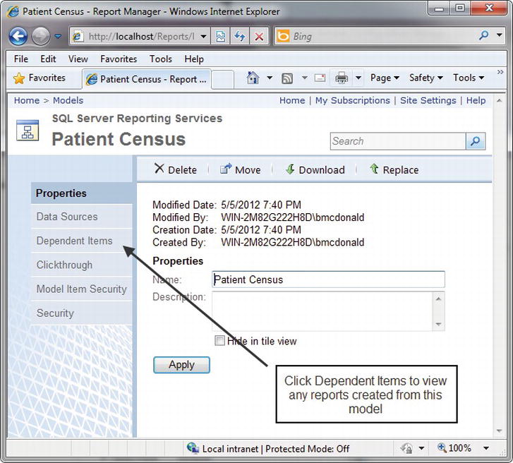
Figure 13-18. Patient Census report model properties

Before you begin creating reports with Report Builder 1.0, it is important to note that users who will need permissions to use Report Builder 1.0 must have item-level role assignments for various tasks associated with creating reports with Report Builder 1.0. Reporting Services includes a Report Builder 1.0 role for this purpose, as shown in Figure 13-19. Users assigned to the Report Builder 1.0 role have all the required permissions to access the report models, folders, and published reports. To publish reports, however, they will need to have the ability to manage report content before they can successfully publish their reports to the report server. The Content Manager role has all the required permissions for full report creation and publishing capabilities.

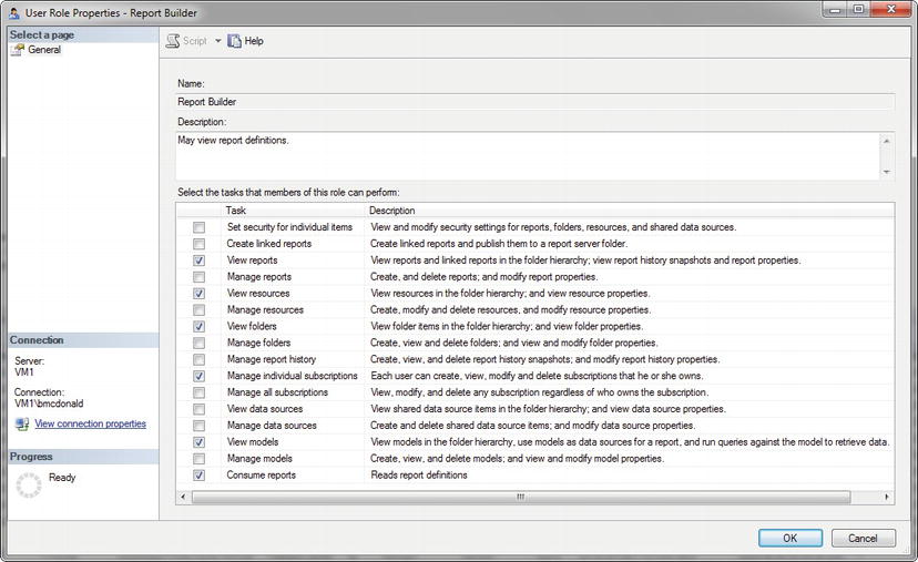
Figure 13-19. SSRS Report Builder role

Creating Reports with Report Builder 1.0

To this point you have created all the requisite pieces for using Report Builder 1.0—you have created the report model Patient Census and deployed it to the report server. It is now waiting to be used as a source for the front-end Report Builder 1.0 application. Report Builder 1.0 provides some of the same functionality of a report development environment, such as BIDS or Visual Studio, including the ability to drag and drop data elements to the design area with Matrix, Table, and Chart data regions as well as the ability to deploy finished reports to the report server. However, before you dive in, we should state that Report Builder 1.0 serves the purpose of allowing end users to design their own reports. It was designed to be intuitive and friendly, and because it is not a full-featured IDE, it may at first seem limited.

In this section, you will explore Report Builder 1.0 and uncover the features that are available to the report designer such as adding functions, similar to adding expressions in BIDS, and providing filtering, grouping, and sorting capabilities. The goal in this section is to show you how to create and deploy, step by step, the requested census reports from the Patient Census model created earlier in this chapter.

When Reporting Services is installed for SQL Server 2008 R2, the default Report Builder application is 3.0. If you are following along or you want to create reports using Report Builder 1.0, you will either need to navigate directly to the Report Builder URL or change the default Custom Report Builder launch URL in the Site Settings section of the Report Manager. You can find the report builder application under the Program FilesMicrosoft SQL ServerMSRS10_50.MSSQLSERVERReporting ServicesReportServerReportBuilder folder. To follow along, we are going to set the launch URL in the Report Manager to use Report Builder 1.0. To do this, open up Report Manager by navigating to http://ServerName/Reports. Once Report Manager is open, click on the Site Settings link in the top right corner. Set the launch URL to:

http://localhost/ReportServer/ReportBuilder/ReportBuilder.application

After you change the default Report Builder URL, now let’s use it. Click Apply to save your changes and navigate to the Report Manager home page. Once on the home page, you should see the Report Builder icon on the main toolbar of the Report Manager as shown in Figure 13-20. Click the Report Builder button to initialize the Report Builder 1.0 installation if it is not already installed or to open the installed application.

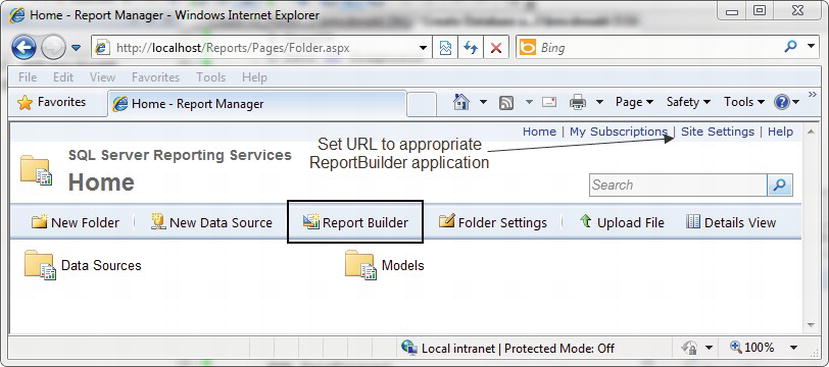
Figure 13-20. Report Manager main toolbar with Report Builder button

Report Builder 1.0 uses ClickOnce technology to install itself from the Web site. The code is downloaded and installed to the local machine from the browser, assuming there are no issues with missing prerequisites, one of which is .NET Framework 2.0. If this is not installed, it will issue a warning message that Report Builder 1.0 requires .NET Framework 2.0 before it can be installed. If all the requirements are met, Report Builder 1.0 initiates and completes installation. Figure 13-21 shows the ClickOnce application installation screen.

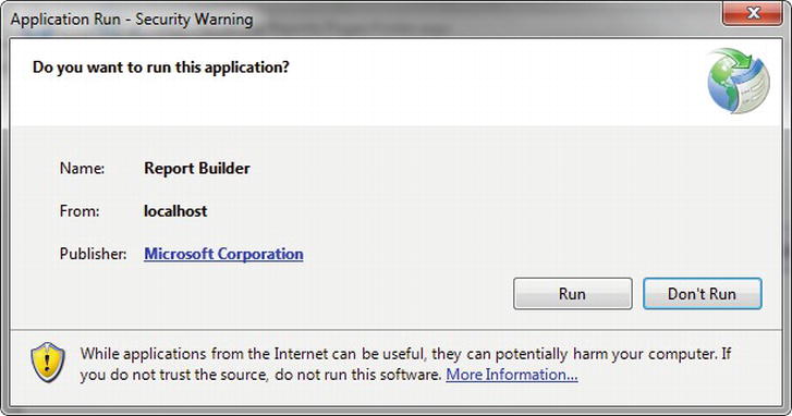
Figure 13-21. Report Builder 1.0 installation progress

After Report Builder 1.0 is installed, it launches automatically. The first step to begin designing a report is to select a source of data, as shown in Figure 13-22. The source will be a report model, in this case the Patient Census report model you have already published. So, select it, and click OK to continue.

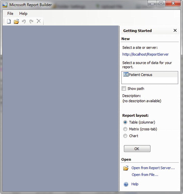
Figure 13-22. Selecting the report model

At first glance, it is easy to see that Report Builder 1.0 has the look and feel of other Microsoft design products in the Office 2007 suite, such as FrontPage. You will see a simple design area, a Report Data area, and a Report Layout area that contains templates that can be used for each report. The three available templates are familiar versions of data regions available for SSRS reports: Table, Matrix, and Chart. Each template has predefined areas such as a title, a total column, and a filter description column, as shown in the table report in Figure 13-23. You can also see the fields of the Patient Census report model in the Report Data tab on the left.

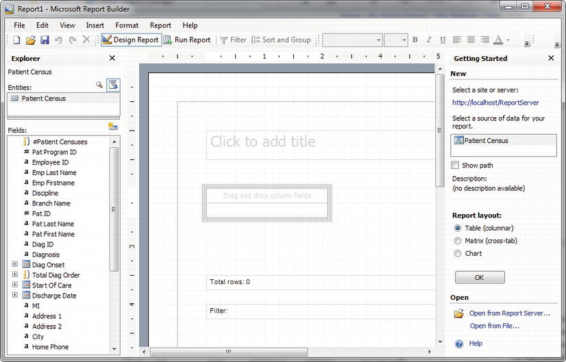
Figure 13-23. Table report template in Report Builder 1.0

Creating a Table Report

To address many of the report requests received from user feedback, you can use the table report. One item to note, which may fall into the category of a limitation of Report Builder 1.0, is that you can use only one data region per report. In other words, unlike the full IDE of BIDS, users who build reports with Report Builder 1.0 are limited to one Table, Matrix, or Chart data region per report. You cannot add a second data region. In fact, reports are not only limited to a single data region, but they are relegated to using the controls that have been defined for each template. It is not possible to add textboxes, for example, or any other type of design element, other than the data from the fields. You will work within this limitation to produce your first report, a patient face sheet (as it is commonly called), which displays demographic information about each patient. With the table report still open, you will drag several fields onto the table where it says Drop Column Fields so that the report looks like Figure 13-24. Next, hold the CTRL key down on the keyboard while selecting Pat ID, Pat First Name, Pat Last Name, Diagnosis, Start Of Care, Address 1, City, State, and Zip. After you have them all selected, drag them to the right of Pat ID in the table of the report. By holding the CTRL key, as we’ve done here, we create a group of Patient Census column names. At this point, you can also add a title in the Click to Add Title textbox. Change the title to Patient Face Sheet and make it bold. Notice also that as the fields are added, Pat Last Name, for example, they become bold in the Fields tab on the left indicating they have already been used.

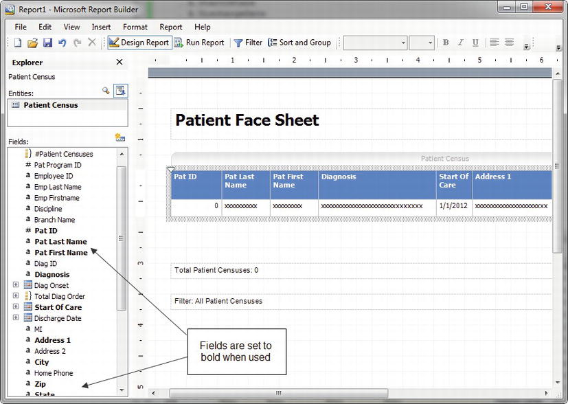
Figure 13-24. Table report with patient information

Once you have added all these fields to the report, you could click Run Report to preview the report; however, at this point, you must perform some tasks to make the report fit on a printed page. In its default page setup, the report is set to Portrait; however, the fields you have added extend beyond 8.5 inches across. To fix this, right-click in the design area, and select Page Setup so that the Page Setup dialog box appears, as shown in Figure 13-25. Set the Orientation property to Landscape, then set all of the Margins to 0 and click OK.

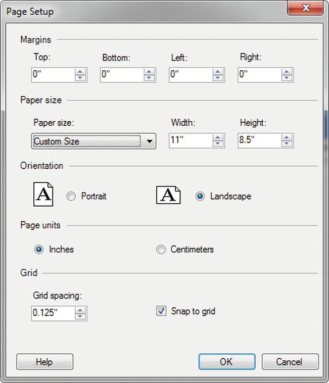
Figure 13-25. Setting the page orientation

To make even more room, you can use a formula to combine the patient’s first and last names. To do this, simply right-click the Pat First Name data cell, and select Edit Formula. This will open the Define Formula window. Formulas in Report Builder 1.0 are like expressions in BIDS. Here is where you can combine report fields and built-in functions to produce the desired value. Figure 13-26 shows the Define Formula dialog box with several available functions. Notice the formula used to concatenate the Pat First Name and Pat Last Name fields, which uses report data fields and an ampersand (&) to add a literal comma character to separate the names. You can also use the RTRIM function to remove trailing spaces. You could have done much of this work in the report model, where it most likely should have been done. However, we had you leave the names this way so we could now demonstrate the use of a simple formula. Once the formula is in place, click the Save this formula as a new Patient Census field, and click OK. You are then prompted to enter the New Field Name. Call this field Patient Name and click OK to save your new field.

Figure 13-26. Define Formula window

Now that you have the patient’s full name combined, you can delete the Pat Last Name field by clicking the data cell and pressing the Delete key. A couple of other tasks remain before previewing the report. The first one is to move the Zip column to the right of the State column. To do this, just click on the cell containing Zip and drag it to the right of the State column. Next, let’s resize the fields so that each record will fit on a single line. Of the fields you have used for the report, the Diagnosis and Address fields have the potential to be the largest, as they are variable-length fields that usually contain between 20 and 50 characters. However, since we want the headers for each column to be on one row, we will also resize Start of Care. For this example, size the Pat ID field to about .5 inches, expand the Diagnosis, Start of Care, and Address 1fields to approximately 1.5 inches, and preview the report, as shown in Figure 13-27. There will be as many x characters representing the data as there are characters found in the largest value in the database field, which makes it easy to determine how much to resize each column. The reason that the Address fields display NA is because this information was either scrambled, in the case of the patient names, or modified to be NA to remove identifiable information. Notice also, in Figure 13-27, that each field automatically contains an interactive sorting icon at the column heading level. Though clicking the icon will re-render the report, no actual sorting will be performed until you configure it to do so. You will do that next.

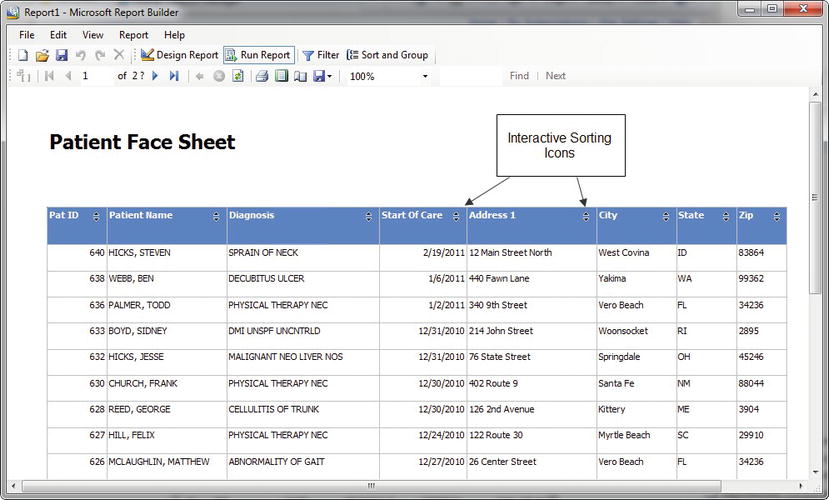
Figure 13-27. Previewing the Patient Face Sheet report

Return to the design area of the report by clicking the Design Report button on the toolbar. Next, right-click the Pat ID data cell, and then select Sort and Group on the toolbar. This will open the Sort dialog box. With the Patient Census group selected, choose to first sort by Pat ID, then by Patient Name, and finally by Diagnosis, as shown in Figure 13-28. You also have the ability to put a page break after each group as a group option. Do not add a page break at this time. Once you click OK, you can preview the report and see that the sorting for each of the defined columns is working correctly.

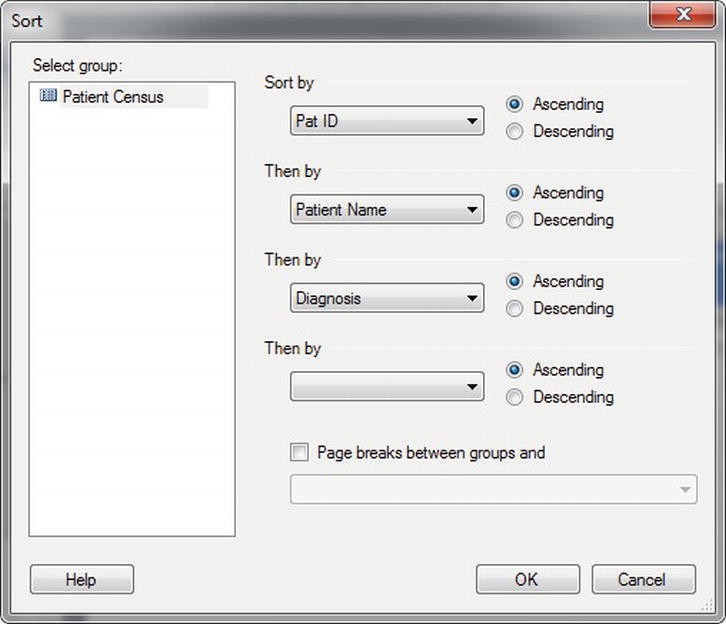
Figure 13-28. Sorting and grouping options

We should mention one more thing about dragging fields to the table area of the report: groups are automatically defined from left to right. In other words, dragging and dropping fields to the right of another field keeps the field in the same group, in this case the Patient Census group; however, if you have already dragged a field to the table and then drag another one to the left of it, another group is created based on the name of the field that is dropped. You can see this in Figure 13-29, where if you were to drag the Branch Name field to the left of the Pat ID field. If you are going through these steps, go ahead and drag the Branch Name field to the report to see the automatic grouping. Also, go ahead and resize the table header row to have a height of one line. Then drag the entire table to be a little closer to the title. Performing these steps should result in a report similar to that shown in Figure 13-29.

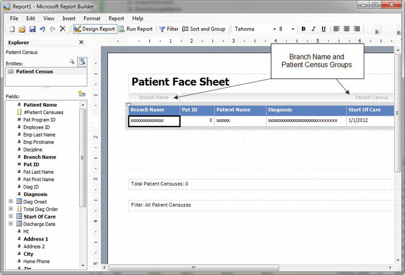
Figure 13-29. Automatically created groups

You can preview the report one last time before saving it to the report server. Notice in Figure 13-30 that the newly added branch group hides duplicate values automatically and groups each record from the Patient Census group under its assigned branch name. You could, at this point, use standard formatting features such as adding a border or changing the background color of cells or even the font size, color, and justification if you so desired, but the base report meets your needs, so go ahead and deploy it.

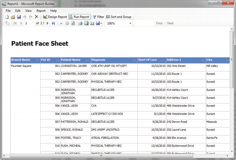
Figure 13-30. Previewing a new Branch Name group

Deploying the report to the report server is as simple as clicking the Save button on the toolbar. After clicking Save, a Save Report dialog box appears that allows you to navigate to an accessible folder on the report server; in this case, open Pro_SSRS folder by double clicking it. If you do not have a Pro_SSRS folder on your SSRS 2008 R2 server, simply navigate to the Report Manager (http://localhost/Reports/) and click the New Folder button on the toolbar of the home screen. Name the folder Pro_SSRS and click OK to create the definition of the new folder in the ReportServer database. Name this report Patient Face Sheet, as shown in Figure 13-31, and click the Save button.

You can navigate to the Report Manager later to make sure the report was saved successfully, but for now, you will move on to the next type of report you will learn how to create, a matrix report.

Figure 13-31. Saving a report to the server

Creating a Matrix Report

Unlike a table report, a matrix report displays aggregated values two-dimensionally with column groups as well as row groups. The totals, whether they are sums, averages, or counts, intersect at the grouping levels for columns and rows. This creates a cross-tab report similar to a pivot table in Microsoft Excel. One of the requests for the report was to show the length of stay for patients, from the time they were admitted to the time they were discharged. It is also a requirement that the discharge reason show on the report. You can combine these two requests perfectly into a single matrix report.

So, return to the Report Builder 1.0 design area, and click the Matrix (cross-tab) report in the Report layout section of the Task Pane. This opens a new blank matrix template where you can drag and drop fields onto the Matrix data region, just as you did with the table report. The template is nothing more than a predefined Matrix data region to which you will add several fields, as shown in Figure 13-32.

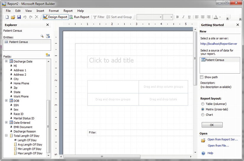
Figure 13-32. Blank matrix report

To start this report, expand the Total Length of Stay attribute in our Fields list. Drag the Avg Length of Stay attribute that was calculated when the model was generated over to the totals area of the Matrix. For the row grouping, add the Discharge Reason field. Finally, drag the Marital Status ID field to the column grouping area so that the matrix report resembles Figure 13-33. It will be necessary to resize the Discharge Reason field and center-justify the Marital Status ID field. You will also at this time add a title to the report: Average Length of Stay. Make the title bold and set the font type to Arial Rounded MT Bold.

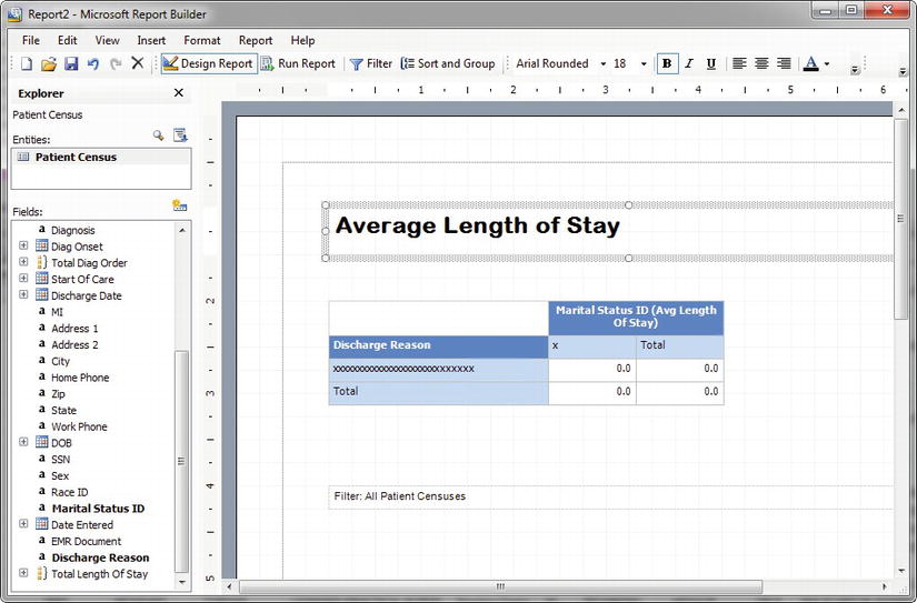
Figure 13-33. Matrix report with data

When previewed, the report is already taking shape, as shown in Figure 13-34; however, you need to address some anomalies. First, the number format is not what you expected or wanted. A general number, which by default is the data type assigned to the Avg Length of Stay field, is not desired. You will need to add formatting to the number. Second, you will see rows and columns with empty values. This is happening for two likely reasons. First, you are including patients who have not been discharged yet, in other words, active patients. Second, marital status is not a required field, so some records will not have values.

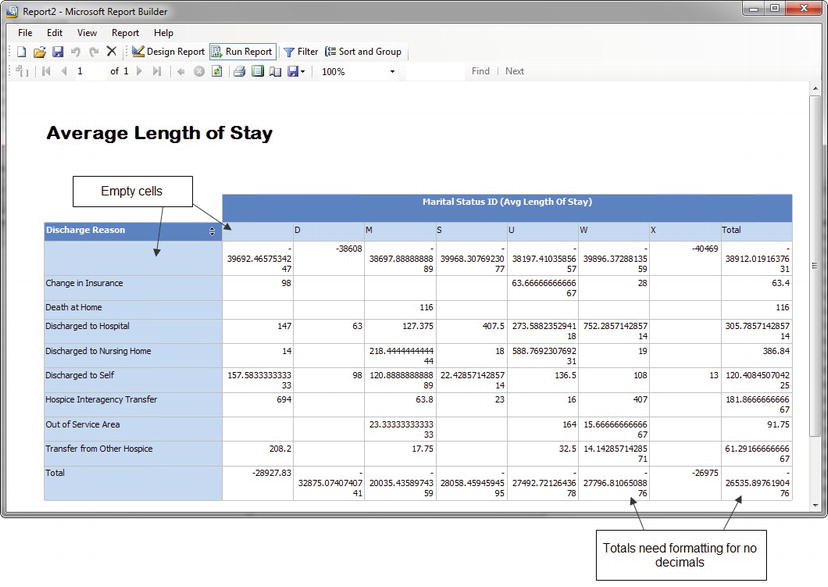
Figure 13-34. Initial preview of a matrix report

You can take care of the number formatting by returning to the design area, right-clicking the last column (which is the total), and selecting Format. In the Format dialog box, change the defined format from General to 1234.56, as shown in Figure 13-35, and change the decimal places from 2 to 0. Then click OK. Perform the same formatting on all of the other value fields.

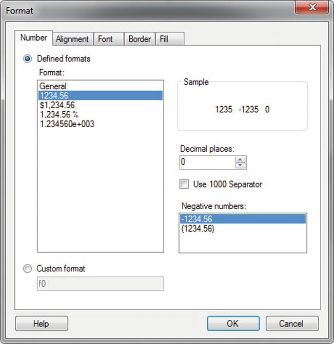
Figure 13-35. Changing the number formatting

To address the empty columns, add a filter to the report to limit the data to only discharged patients with discharge reasons and to patients who have a marital status defined. The Filter button on the toolbar will launch the Filter Data dialog box. In Figure 13-36, you can see that you can add four filter conditions: where MaritalStatusID, Discharge Date, and Discharge Reason are not empty and where the Discharge Year is greater than or equal to 2010. (We added the last filter to demonstrate that it is possible to have the report prompt the user for a value as a parameter that is tied to a filter.) To change the comparison operator from the default of equal to not empty, click on empty and select both Not and Is Empty from the available operators. For the Discharge year, select the Greater Than or Equal To operator. After you set the year to be 2010, click on the Discharge Year label and select Prompt to set it as a report parameter as depicted by the green question mark icon shown next to the Discharge Year filter label.

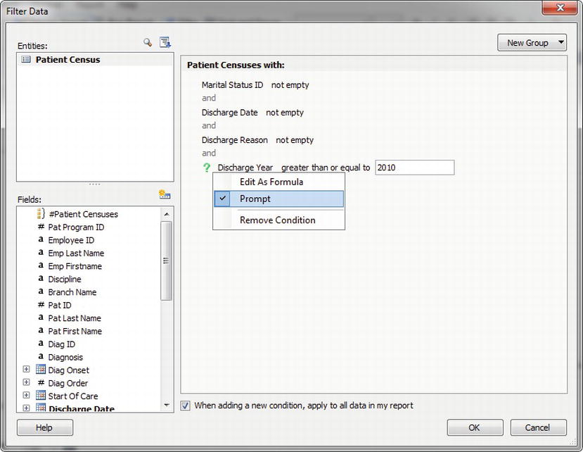
Figure 13-36. Setting up report filters

Now, when you preview the matrix report in Figure 13-37, you can see that the numbers have been cleaned up and all empty fields are gone; also, you are prompted for the discharge year. Change the Discharge Year parameter to 2011 to see those results. Save the report as Average Length of Stay to the Pro_SSRS folder on the report server, just as you did the table report. We will now move on to create the final report using Report Builder 1.0, the chart.

Figure 13-37. Setting up report filters previewing the report

Creating a Chart Report

The last report type available in Report Builder 1.0 is the chart report. Thus far, you have created and saved table and matrix reports to address many of the report requests for the Patient Census report. Now, we will show one of the most important reports to answer the question of the number of patients on the census. Census means that the patients are currently receiving services and have not been discharged. In the database you are using, a patient is considered active if his or her discharge date is Null, or, in Report Builder 1.0 vernacular, empty. The chart you create will be a simple bar chart showing a count of active patients by their branch association.

Return to the design area of Report Builder 1.0, and click the chart report in the Report Layout tab. The blank report template has a single Chart data region, as shown in Figure 13-38. As you did with the two previous reports, table and matrix, you will add a title: Active Patient Census.

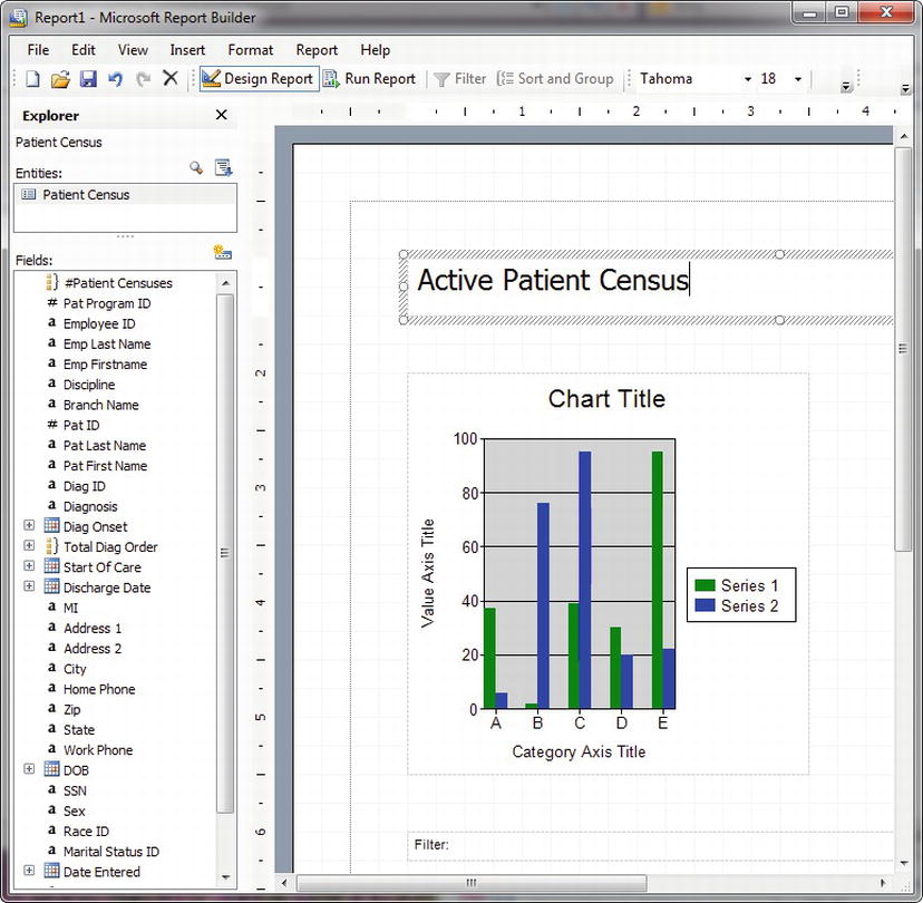
Figure 13-38. Chart report template

The chart has three areas to which you can drag and drop data: Series, Category, and Data. You want to be able to show an active patient count, so you could drag the Pat ID field to the Data area; however, because the Pat ID field is not seen as a field that can have an aggregated function applied to it, unlike Avg Length of Stay, you cannot drag it directly to the Data area. The chart simply won’t accept it to be dropped there. Since you know you will need both a count value and a filter to get only active patients, you can take care of both at the same time by adding a new field to the field list. Click the New Field button in the Explorer tab, and name the new field Patient Count, as shown in Figure 13-39. The formula you can use for the Patient Count field is COUNTDISTINCT(Pat ID). Notice that in the Define Formula dialog box that the Pat ID field, when added to the Formula textbox, has a dotted line beneath it indicating a link. You can click the field and add a filter while defining the formula for the new field, which you will do next.

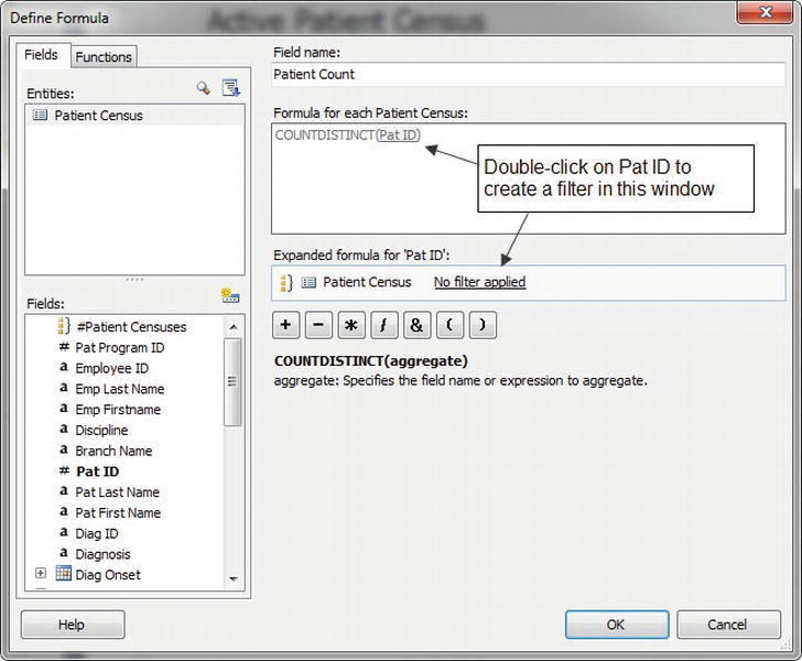
Figure 13-39. Defining a formula for a new field, Patient Count

Click the No Filter Applied link, and select Create a New Filter to open the Filter Data dialog box. You can see the filter you need to apply to show only active patients in Figure 13-40, where you have set Discharge Date to “empty,” which will force only patients who do not have discharge dates to be used in the formula. To implement the filter, drag Discharge Date over into the filter pane. Then select the Is Empty value by clicking on the equals link label. Call the filter Active Patients, and click OK. Once the Patient Count field is created and shows up on the Fields tab, you can drag and drop it in the Data value fields area of the chart. In this case, since we are adding it to the Data value fields area, we could simply double-click on the Patient Count field and Report Builder will place it in the correct section.

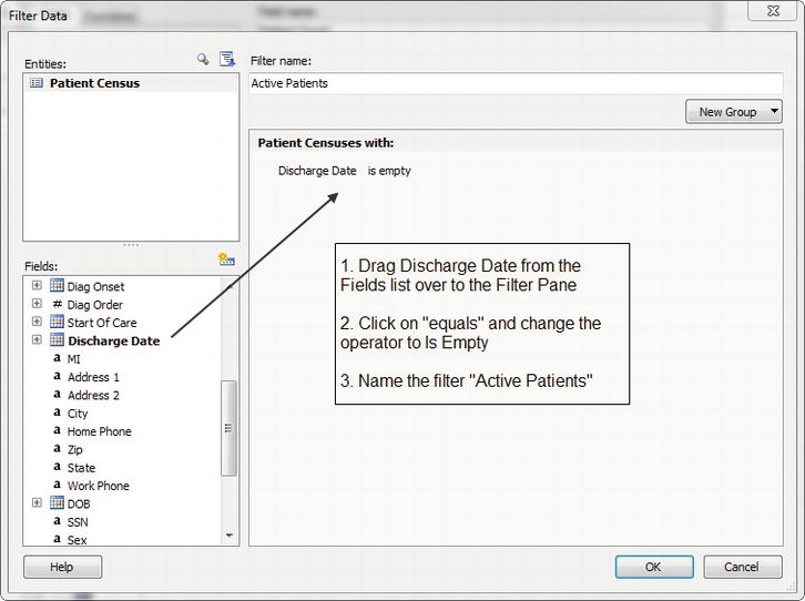
Figure 13-40. Adding the Active Patients filter

Next, drag the Branch Name field to the Categories area of the chart. You could add further series items or categories to the chart, but to keep the chart simple and to address the request, you will just apply some formatting to the chart by way of removing the chart title so that it does not say “Chart Title” on the report. To modify the chart properties, follow these four steps:

1. Right-click the chart, and select Chart Options.
2. On the Titles tab, delete the text for the chart, Category X and ValueY titles.
3. On the Legend tab, remove the check from the Show legend checkbox.
4. Finally, on the 3D tab, check the Display Chart with 3-D Visual Effect box, set Horizontal Rotation to 25, set Vertical Rotation to 10, Realistic as the Shading, and select Cylinder as the shape, as shown in Figure 13-41.

Figure 13-41. Setting 3D visual effects

The last task before previewing the report is to set the data labels on the chart. To do this:

1. Right-click the chart, select Data Series, and then select Format Data Series–Patient Count. If you would like to have the patient count value display on the bars of the chart, select Show Point Labels. For this example, select the option to Show point labels.
2. Set the angle to –10 degrees to make it stand out a little.
3. Click the Format button to set the font size to be 16.

When you click OK to set the point labels and then preview the report, you can see the chart with the active patient counts per branch. As patients are discharged, they will drop from the active patient list because of the filter, and the chart will automatically reflect the current census count. Figure 13-42 shows the completed chart. Now you can save the chart report as Active Patient Census to the Pro_SSRS folder, as you did the other two reports.

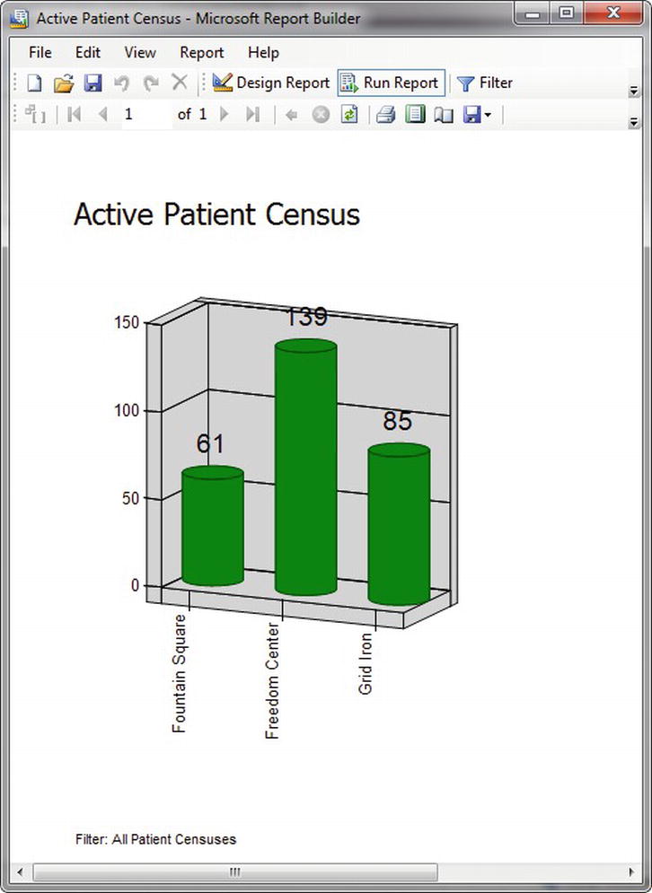
Figure 13-42. Preview of the Active Patient Census chart report

The reports are deployed as standard RDL report files with the exception that their data source is a report model and not a standard RDS data source object. You can see the three newly published reports in Report Manager, as shown in Figure 13-43.

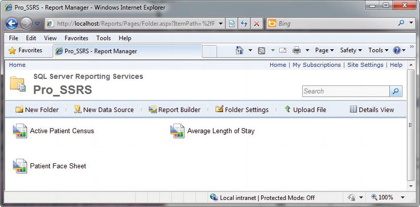
Figure 13-43. Report Builder 1.0 reports published in Report Manager

Creating Reports with the Report Builder 2.0 Wizard

At this point, we created SSRS reports with BIDS and Report Builder 1.0 using ClickOnce. Both design environments provide different levels of control over report design. While BIDS offers report creators much more flexibility than Report Builder 1.0, it might not be the best choice for people who are not also application programmers. Report Builder 1.0, by contrast, is easy to learn and to use to publish reports; however, it comes with limitations in that reports can only be created using prebuilt models, which is not enough to meet everyone’s needs. In SSRS 2008, Microsoft provided Report Builder 2.0, which supported true ad hoc query and report design not solely based on report models. Report Builder 2.0’s modern look and feel, with Ribbon technology like that found in Office 2007 applications, gave report creators a familiar environment to work in.

Figure 13-44 shows the Report Builder 2.0 interface. Microsoft’s use of the new Ribbon technology is apparent in the figure.

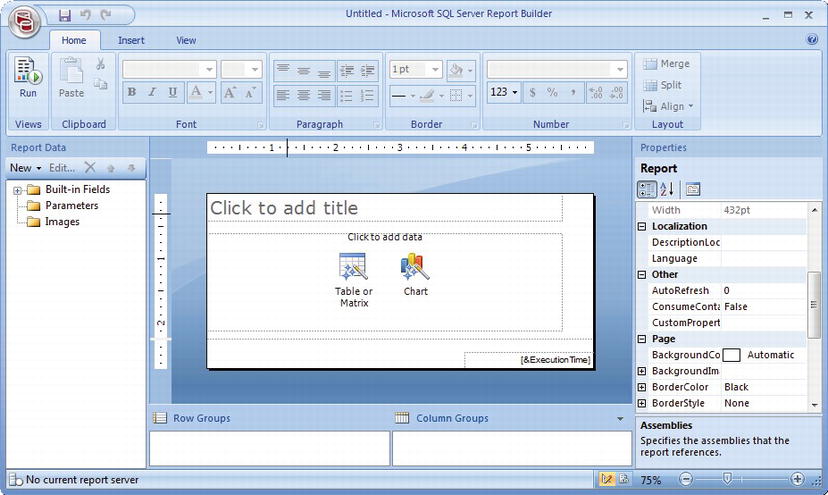
Figure 13-44. Report Builder 2.0’s new interface

As you might imagine, developing a report in Report Builder 2.0 is simplified, with all design choices available in one of three tabs, Home, Insert, and View. Built-in fields, parameters, images, and data sources are all contained in folders within the Data window. Like in SQL Server Data Tools (SSDT), Row Groups and Column Groups areas located are on the bottom. Instructional text, as well as link buttons that fire up the Table, Matrix and Chart wizards, have been added to the body of the report to guide the designer through the required steps to producing a finished product.

By way of example, let’s build a new version of the Employee Service Cost report that you’ve been seeing throughout this book. If you are using SQL Server 2008 R2 or SQL Server 2012 and using the Report Builder 2.0 from installing the thick client as I am, you will start Report Builder 2.0 by navigating to the Microsoft SQL Server 2008 Report Builder 2.0 folder under All Programs of Windows start menu. Once you have Report Builder 2.0 fired up, you will want to click on the Table or Matrix icon on the report design surface. As mentioned, this will bring up the New Table or Matrix wizard and begins by prompting you to select an existing data source or create a new one as shown in Figure 13-45.

Figure 13-45. New Table or Matrix wizard in Report Builder 2.0

Select New… to create a new data source for this report. Name the data source Pro_SSRS and with the connection type set to Microsoft SQL Server, click on the Build…button to select the server. In this case, set the server name to localhost, Pro_SSRS as the database name, as in Figure 13-46. Click OK to save the Connection Properties and then click OK again to save the Data Source Properties. Now that our data source has been created, click Next to build the query in the query designer window.

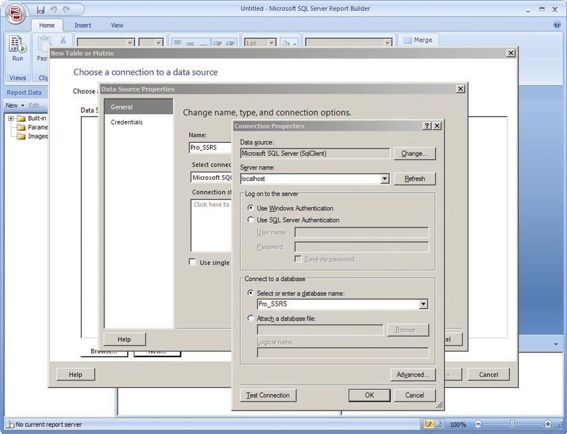
Figure 13-46. Setting data source and connection string properties

The query designer contains a minimal set of tools for query design and is similar in fashion to query builder applications in SSMS. You can graphically add tables to a query, use stored procedures, table valued functions, create joins, and filter data with criteria. In our case, we are going to use the Emp_Svc_Cost stored procedure. In the query designer, we can expand Stored Procedures in the Database view pane and then select the Emp_Svc_Cost stored procedure. As you can see after selecting the stored procedure, you are shown the fields that the stored procedure returns as well as the parameters that the stored procedure expects. If you want to see the Query results, set the parameter values that you want to set and then run the query. For this example, leave the default values set to (null) and execute the stored procedure by clicking the Run Query button. Figure 13-47 shows the stored procedure Emp_Svc_Cost being executed with resultant data. Alternatively, we could have clicked on the Edit As Text button, selected Stored Procedure as the type and then entered Emp_Svc_Cost in the query text box.

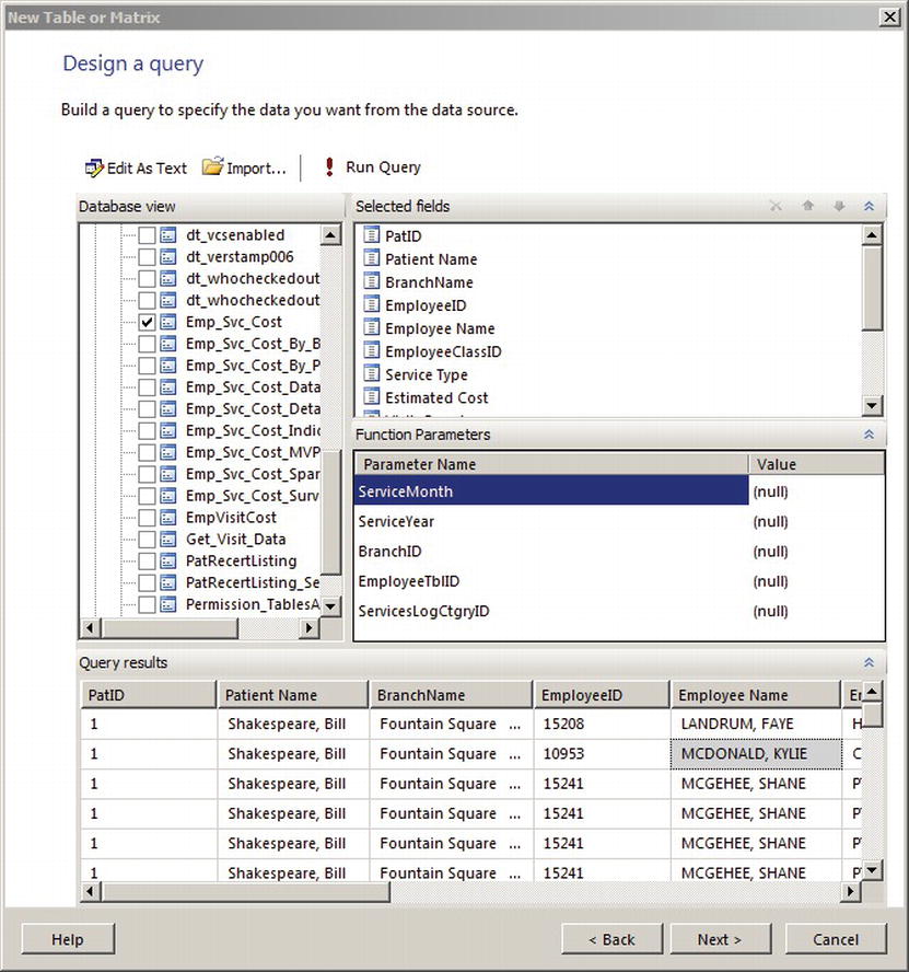
Figure 13-47. Adding the Emp_Svc_Cost stored procedure to query designer

After seeing the results, click Next to progress to the Arranged fields screen of the New Table or Matrix wizard. Here is where you layout your report with the appropriate row groups, column groups and values. Use the following steps to produce the Emp_Svc_Cost report using the wizard:

1. Drag the BranchName and Service_Type fields over to the Row groups area.
2. Next, Drag Visit_Count and Estimated_Cost over to the values area as seen in Figure 13-48.
   

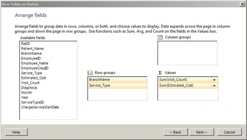
   Figure 13-48. Arrange fields screen

3. Click Next to proceed to the Layout selection screen. This screen allows us to select a blocked or stepped look for our report. It also has a feature for auto creating expanding or collapsing drill down capabilities using the Expand/collapse groups checkbox. Leave the default values as shown in Figure 13-49 and click Next.
4. Leave the default Ocean style selected and click Finish to generate our report.
5. Adjust the columns to a width that prevents the header contents from wrapping to the next line.
6. Change the title to Service Type Estimated Cost by Branch.

Figure 13-49. Choosing a report layout

With these minor changes performed, we should have a report similar to what is being shown in Figure 13-50.

Figure 13-50. Finished report in Report Builder 2.0

Save this report out to the Pro_SSRS folder on the Report Server as in our previous examples and name it Service Type Estimated Cost by Branch Wizard. In the sections that follow, we’ll walk through another way to create the same report without using the wizard. We will also show you how to perform format changes to the Report Builder reports.

Creating Reports with Report Builder 2.0

As I just mentioned, we do not have to use the wizard when creating reports. Alternatively, if we didn’t want to utilize the New Table or Matrix wizard, we could create a new data source and dataset separately. In this section, we are going to create the same report without using the wizard.

To get started, if you have the Service Type Estimated Cost by Branch report still open, click on the circular ribbon icon on the top left of the screen. This ribbon icon, acts as the File menu option in other Microsoft products. After clicking on the ribbon icon, select New to create a new report. If you do not have Report Builder 2.0 open, navigate to the Report Builder thick client under the Microsoft SQL Server 2008 Report Builder 2.0 from the All Programs menu. If you have been following along, the blank design environment of Report Builder 2.0 should look familiar to you as it is the same as shown in Figure 13-44.

To get started on creating a report from scratch without using the wizard, we will need to create a data source and a data set before getting to the report design. After we have these created, we will be able to add a table to our design pane and then start adding columns and groups. The following four steps will walk us through create the data source and dataset for our report.

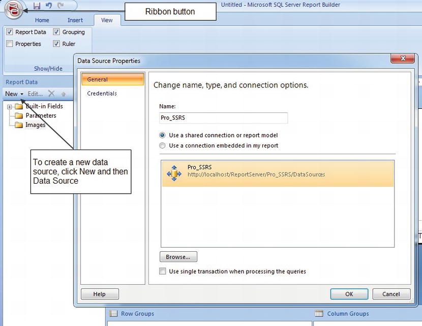
1. Click on the New button on the Report Data pane and then select Data Source. If you do not see the Report Data pane, click on the View tab and then select the Report Data checkbox.
2. Name your data source Pro_SSRS and set the Use a shared connection or report model option. Instead of having an embedded data source, we can use a shared one on the server. This helps when deploying reports to different environments. If the reports use shared data sources, if the database server is changed during the lifecycle of the report, the only object that will require updating is the shared data source itself. Conversely, if you always use embedded data sources, each of the reports that utilize the data source would also need to be changes. This makes it harder to manage and as such, one should use shared data sources when possible.
3. Now, select the Browse… button to navigate to the DataSources folder under the Pro_SSRS folder and select the Pro_SSRS data source. Click Open to return back to the Data Source Properties window as shown in Figure 13-51. Click OK to save the Pro_SSRS data source to return back to the Report Builder. After you save the data source, Report Builder adds it the Report Data pane.
   

   Figure 13-51. Creating a new data source

4. Right-click on the new Pro_SSRS data source in the Report Data pane and select Add Dataset. Name the dataset Emp_Svc_Cost and set the Query type to Stored Procedure. If prompted for login credentials, enter the appropriate login details. Then in the Select or enter stored procedure name drop down, select our Emp_Svc_Cost stored procedure. Figure 13-52 displays the Data Properties window. Click OK to save the Emp_Svc_Cost dataset.

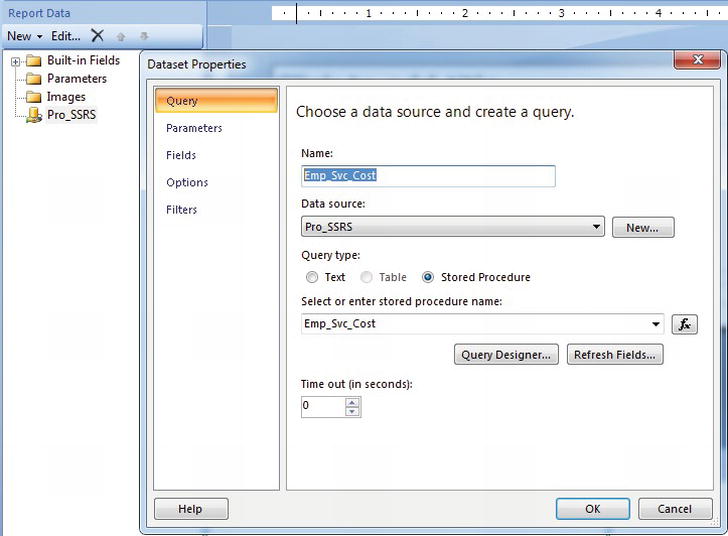
Figure 13-52. Creating a new dataset

Once a query has been added and the data source saved, you can see the available fields as well as the parameters that were automatically generated that can now be used in the report. Also, the directional text in the report has changed. As shown in Figure 13-53, you are now instructed on how to add an item to the report body, page header, and/or page footer by clicking the Insert tab or dragging an item to the appropriate area. You will do that next by adding a Matrix control to the report body, a report title to the page header, and the report execution time, a built-in field, to the page footer.

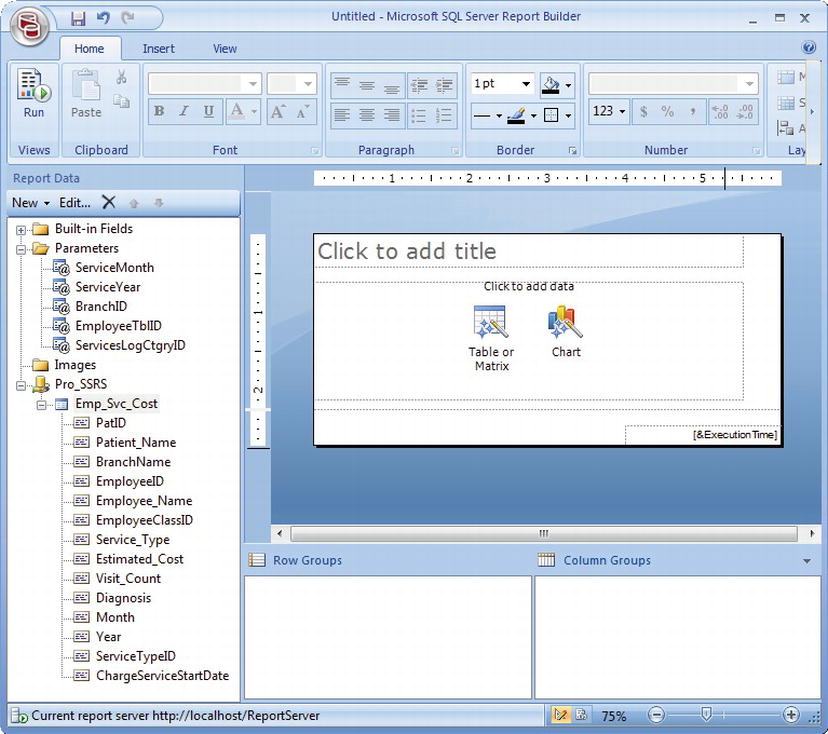
Figure 13-53. Report Builder 2.0 after adding data source and dataset

Now that you have the environment ready to create a report with the newly added data source, click the Insert tab. As you can see in Figure 13-54, all of the report controls are available in four categories at the top: Data Regions, Report Items, Subreports, and Header & Footer. Before we add our own Table, Matrix, or Chart to the design surface, we are going to delete the Data Region Group that contains the two link buttons for the wizards. Just select the DataRegionPlaceholder and hit the Delete key on your keyboard. To add the Matrix data region, simply click the Matrix icon and choose Insert Matrix to add the control to the body of the report. Next, just draw the Matrix onto the design surface to be approximately ½ inch high by 2 inches long.

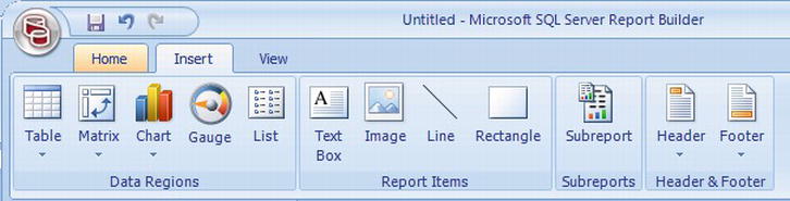
Figure 13-54. Report objects available from the Insert tab

Next, drag the following four fields from the Emp_Svc_Cost dataset that was created with the data source, onto the Matrix control in the report: BranchName, Service_Type, Visit_Visit_Count, and Estimated_Cost. Add BranchName and Service_Type to the Rows area and Visit_Count and Estimated_Cost to the Data area. When we added Visit_Count to the Data area, Report Builder added a header automatically. We don’t want it to be labeled with Visit Count, so select the textbox and then hit Delete to remove it. At this point, the report should be similar to the layout depicted in Figure 13-55. Notice that the Sum functions were automatically applied to the fields dragged to the Data area.

Figure 13-55. Report Matrix with fields added

You will want to resize the cells in the Matrix so that the Service_Type records do not wrap. If you click the View tab, there is a selection for Ruler. Click the Ruler button and size the Service_Type cell to be two inches. Before running the report, let’s change all of the parameters to allow NULL values. To set the parameters to accept NULL values, simply double click the parameters and enable the checkbox labeled Allow null value. You can see the previewed report taking shape (Figure 13-56) by clicking the Preview button, available on the Home and View tabs.

Figure 13-56. Preview of Report Builder 2.0 report

Next, you will format the Estimated_Cost field to display the value as currency. Click back in the Design area, and then follow these steps to apply some formatting:

1. Right-click the SUM(Estimated_Cost) textbox and choose Textbox Properties.
2. Figure 13-57 shows the dialog that presents the textbox properties encompassing many of the formatting and actionable items available, such as interactive sorting, visibility, and hyperlink options. These are all the same as properties that you would set when developing a report in BIDS. Click Number on the left and choose Currency for the format, then choose the option to Use 1000 separator (,) and click OK to save the Textbox Properties.
3. Next, apply the number formatting with the thousands separator to the Visit_Count field by right-clicking it and selecting Textbox Properties. Select the Number tab and then choose Number as the Category. Set the decimal places to 0 and select the option to Use 1000 separator (,) and click OK to save the Textbox Properties.
4. Since the default height of the report has given extra white space, let’s cut down on this by dragging the footer bar up closer to our Matrix report item.
   

   Figure 13-57. Textbox properties for Estimated_Cost

5. Finally, reset the report title by clicking the Click to add title textbox at the top of the report. Set the report title to Service Type Estimated Cost by Branch and change the width of the textbox to be approximately 5 3/4 inches.

When you are done making all of these changes, the report should look like Figure 13-58.

Figure 13-58. Report with title added

Finally, you have probably noticed the [&ExecutionTime] in the report footer. This is added by Report Builder 2.0 by default. If you wish to delete it, just select it and hit delete. However, if you want to add more built-in fields to the footer or header sections, just expand the Built-in Fields folder in the Data window to see your options. You will see ExecutionTime, PageNumber Report Folder, Report Name, Report Server URL, Total Pages, User ID, and Language as possible selections. For our example, we are going to add a header to our report and add the User ID to it along with our report title.

1. While in design mode, click on the Insert tab.
2. Click on Header and then Add Header. Resize it to be about ½ of an inch in height.
3. Select the title in the body of the report and drag it into the header section
4. With the report title selected, click on the View tab and put a check in the Properties option to show it.
5. Change the FontSize property to 14pt rather than the default 20pt. Resize the header textbox to be slightly larger than the title. This will give us some room in our header to show one more field.
6. Drag the User ID build-in field over to the right of the report title. This will create a textbox with the User ID field value. You can right align this new textbox make it italicized and add bold formatting.

You can easily add more formatting, or report beautification as I like to call it, but at this point, the report should look like Figure 13-59 when previewed.

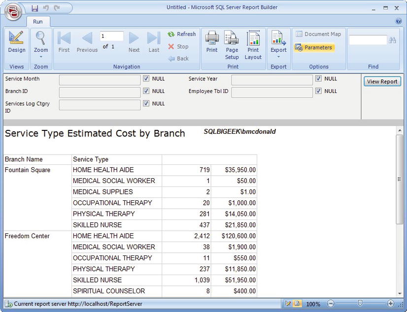
Figure 13-59. Preview of report with execution time and title

For a final touch, you will add totals to the report. This is easily accomplished by clicking back in the design area and selecting both of the cells in the Data region, Visit_Count, and Estimated_Cost. You can select both at once by selecting the first cell and, while holding down the Shift key (or CTRL key), selecting the second cell. Once you have selected it, right-click and then choose Add Totals. The total fields are automatically added for you. You can emphasize the totals by making the two new total cells bold. When complete, the report will appear as it does in Figure 13-60.

As you have seen, the new Report Builder 2.0 has many of the features of the full-blown design environment in BIDS with only minor exceptions. One exception that stands out is the inability to check a report directly into a version control application such as Team Foundation Server.. However, for its intention, the Report Builder 2.0 does serve the purpose of putting a design environment in the hands of people who can create reports beyond the constraint of report models, but who may not be VB .NET developers per se. Making this valuable design tool available as part of SSRS was one more step forward in bringing SSRS to the masses. In the next section, we will cover the enhancements made in the Report Builder 3.0 application as well as walk through an example using the latest release of Microsoft’s Reporting Services ad-hoc tool.

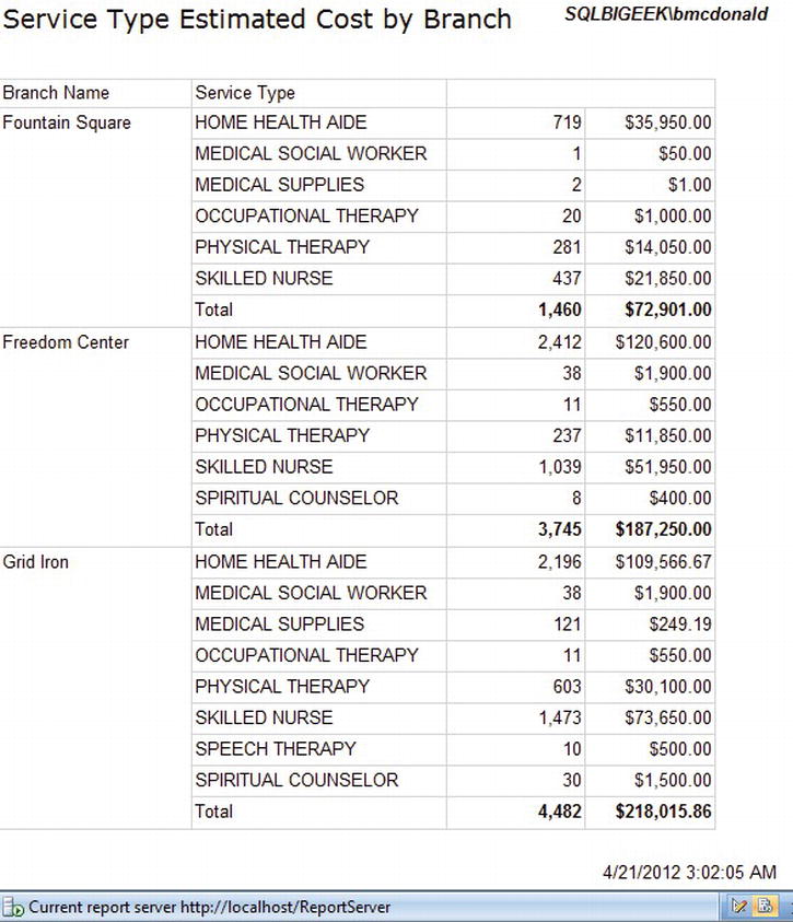
Figure 13-60. Report with final formatting

Creating Reports with Report Builder 3.0

When we heard that SQL Server 2008 R2 was coming to the market with all of the new visual enhancements, there was talk about another Report Builder. After all of the great additions made with Report Builder 2.0, we could not wait to see what ad hoc goodies the next release would bring to our end users.

When SQL Server 2008 R2 came to the market, along came Report Builder 3.0 and with it came some additional data sources, data visualization report items, and cached data sets when previewing reports to name a few. High-level details about each of the enhancements are:

• Report Parts: Report Parts allow report authors to create and deploy reports that can be re-used by other reports. For example, if a report developer created a chart for Employee Service Cost by Branch report with a total cost chart, another report developer or end user could use that report as a Part of their report.
• Data Sources: With the coming of age of SQL Azure, Microsoft has created a Microsoft SQL Azure data source. They have also added the SharePoint List Data Extension to connect to SharePoint lists and Microsoft SQL Server Parallel Data Warehouse.
• Report Items: As discussed in Chapter 5 using the Report Designer in SQL Server Data Tools, new report visualization items have been added to the Report Builder. The new report items are Map, Data Bar, Sparkline, and the Indicator. You can find these on the Insert tab of Report Builder.
• Dataset Caching: With end users creating ad hoc reports, the potential for many long running report requests is pretty high. As such, to prevent multiple round trips when no dataset related changes are made, Microsoft has added dataset caching to the matrix of new features. This makes the end users experience better when creating ad hoc reports, which could equate to more acceptance by end users.

Now that you’ve been introduced to Report Builder 3.0 and some of the new features and enhancements, let’s get started on some examples. In this example, we are going to build a report that has the number of visits and the estimated cost of service for each patients State and by the State in which the patient was seen at one our branches. It will be very similar to the report that we have created with the exception that we will also be using a Map control. We will also have a drill through report from our Map report to a more detailed tabular report. We have learned about drill through reports earlier in the text, but we never performed a drill through using Report Builder. The drill through report demonstrated in this section is available in the Pro_SSRS project in the Source Code/Download area for the book on the Apress Web site (www.apress.com). This report is called Emp_Svc_Cost_By_Patient_State_RB3_Drill.

Before we get started on Map report, open up Report Builder 3.0 from the Report Manager. Once Report Builder is loaded, click Open in the Getting Started window. Navigate to the location where you have the Pro_SSRS solution stored on your hard drive and select the report named Emp_Svc_Cost_By_Patient_State_RB3_Drill. Click Open to open the report in Report Builder 3.0. If you click Run, you should have similar results to what is shown in Figure 13-61.

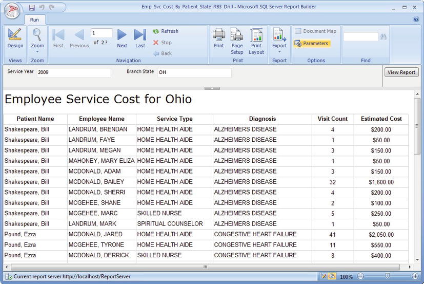
Figure 13-61. Report Builder 3.0 drill through report

After you preview the report, return to the designer and save the report out to the Pro_SSRS folder, as we have throughout this chapter. Saving the report in this path will allow us to drill through to this report when we have our Map report created. With the report saved to the Report Server, click on the Ribbon button and click New. As stated previously, our next report is going to contain aggregated visit and estimated cost for each state that a patient is from as well as which state the patient was actually seen at. Figure 13-62 shows an example of the report while in design mode.

Figure 13-62. Employee Service Cost by branch and patient state in design mode

1. Right-click on the Data Sources folder and select Add Data Source. Name the data source Pro_SSRS, select Use a shared connection or report model and click the Browse button to navigate to the Pro_SSRS data source under the Pro_SSRS/DataSources folder. Click Open and then OK to save the data source.
2. Right-click on the Datasets folder and select Add Dataset. Name the data set Emp_Svc_Cost_RB3 and select Use a dataset embedded in my report. Select the Pro_SSRS as the data source to use and select the Query type radio button to Stored Procedure. Select the Emp_Svc_Cost_By_Patient_State_RB3 stored procedure and click OK to save your dataset.
3. Next, change the report title to Employee Service Cost by Branch and Patient State. Resize the title textbox to fit the new title without wrapping to the next line.
4. Right click on the report design surface, select Insert and then Matrix. This adds a new Matrix report object to the report design pane. Drag the Matrix toward the top left near the title.
5. Drag the Visit_Count field into the Data field and then drag the Estimated_Cost field to the right of Visit_Count.
6. Delete the Visit_Count label that Report Builder put in the Matrix Column field when we dragged Visit_Count over onto our Matrix.
7. Drag the PatientStateName field into the Rows field of our Matrix to create a row grouping for each of the Patients States. Delete the Patient State Name label that was placed in the top left corner of the Matrix as we did for the Visit Count label in step 6. Using the Border Lines formatting option, set the lines around the empty top left corner field to be None.
8. Insert a Rectangle report object in the Columns field by right-clicking in the columns field, selecting Insert and then Rectangle. This is where we are going to put the BranchStateName and a Map for the State. So that we have some room for our BranchStateName and a Map, make the height of this row to be about 2 inches as shown in Figure 13-62 shown previously.
9. Right-click inside of this new Rectangle, select Insert, and then Textbox. Move the Textbox to the top of the Rectangle and set its width to be 2.5 inches. Right-click the textbox and select Expression. Set the expression so that it reads Fields!BranchStateName.Value. Click OK to save the expression. Center the alignment of the text and make it Bold. Then enter a space after the [BranchStateName] and then enter Branch. The textbox should now read [BranchStateName] Branch.
10. Select a blank section in the Rectangle just below the BranchStateName textbox that we just created. Using the Home tab on the Ribbon, change the color of the lines surrounding the rectangle to be Silver and then click on the border to place lines around the entire rectangle. At this point, our report should look similar to Figure 13-63.
    

    Figure 13-63. Employee Service Cost by branch and patient state

11. Format the [Sum(Visit_Count)] field to be Number with no decimal places by selecting the field and then selecting the Properties on the View menu. Navigate to the Format property under the Number category. Set the format to be N0 (that is N and zero). Center the field.
12. Format the [Sum(Estimated_Cost)] field to be Currency with two decimal places by setting its Format property to C2.
13. Add a row above the PatientStateName, Visit_Count and Estimated_Cost row by right-clicking on the PatientStateName field, selecting Insert Row and then Outside Group – Above. Now that we have these extra fields, let’s put labels in them to represent the columns that are below them. Set the first empty textbox to read Patient State, the second to Visit Count, and the last one to Estimated Cost. Make each of the fields Bold and widen the Patient State column to be about 1.75 inches wide. Click Run to see the fruits of our labor up to this point. Set the Service Year parameter to 2009 and click View Report. Figure 13-64 shows what the report should look like if you have been following along.
    

    Figure 13-64. Previewing Employee Service Cost by branch and patient state after outside group and formatting

14. As you can see, we have left some space below the branch State names textbox and the new group. Now we are going to add a Map to that empty space. Click on the Design button to return to the Report Builder designer.
15. Right-click in the empty space below the BranchStateName textbox, select Insert and choose to insert a new Map report object. Report Builder will make the rectangle much larger, but we will shrink it down after we get the Map just the way we want it.
16. To get started, we are going to remove the extra items that are added by. Right-click on the Map and remove the checkbox from Show Meridians. Do it again to remove the checkbox from Show Parallels. Perform the same action for the Color Scale (bottom left) and the Distance Scale (bottom right). Right-click on the legend and then select Delete Legend. Perform the same action for the Map Title, At this point, the Map looks like a giant grey rectangle right? I would say that we are all done, but that would be a joke. In actuality, now we are ready to work some mapping magic.
17. Right-click the map, select Map, and then Add Layer. Leave the default Map Gallery selected, choose the USA by State Inset, and then click Next. We will set the zoom to be dynamic later on, so for now, click Next on the Choose spatial data and map view options screen to progress through the New Map Layer wizard. Choose the middle option, Color Analytical Map and click Next. We could create a new dataset or browse for another one, but we already have one that we can use. Select our Emp_Svc_Cost_RB3 dataset that already exists in our report and hit Next. In the Specify the match fields for spatial and analytical data screen, put a checkbox in STATENAME, and then select BranchStateName as the Analytical Dataset Field to map to Click Next. Set the Theme to Generic, Field to Visualize to BranchStateName, and click Finish to complete the map layer wizard.
18. Click on one of the States to bring up the Map Layers box and click on the down arrow next to the image of the eye. Select Polygon Color Rule. For this example, we are going to choose the option to Visualize data by using custom colors. Next, click the Add custom colors button and set the color to be Sea Green. Click OK to save the Map Color Rules Properties.
19. Resize the map to be the same width of the BranchStateName textbox and approximately 2.5 inches in height. Resize the width of the column that contains the map to be about 2 inches wide. Set the height of the row containing the map to be around 2.5 inches.
20. Right-click on the map and select Viewport Properties. Navigate to the Fill tab and set the Fill style to be Solid. Click on the Border tab and set the Line style to None. Click on the Shadow tab and set the Shadow offset to be 0pt. Now to have the map dynamically zoom into the State, click on the Center and Zoom tab. Change the setting to Center map to show all data-bound map elements and set the zoom level to be 1000. Click OK to save the Viewport Properties.
21. Expand the Parameters folder in the Report Data pane. Next we’re going to add a few year values for our ServiceYear parameter. Double-click on the ServiceYear parameter to open its properties window. Click on the Available values and select Specify values. Click the Add button three times to hold three different values. For the first value, enter 2009 as the Value. Enter 2010 for the next one and 2011 for the last one. Click on the Default Values tab and choose the option to Specify values again. Click the Add button and set its value to be 2009. Click OK to save the Report Parameter Properties. The report should closely resemble what is shown in Figure 13-65.
    

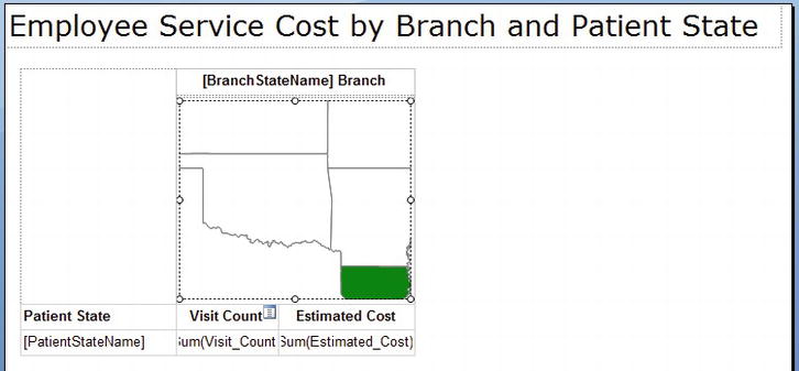
    Figure 13-65. Employee Service Cost by branch and patient state after outside group and formatting

22. We are almost complete! One final requirement is to have the ability to drill through from this report to our detailed report named Emp_Svc_Cost_By_Patient_State_RB3_Drill that we deployed earlier. To do this, we are going to create an action on the map. To do this, click on a State again to bring up the Map Layers window. Click on the down arrow as you did earlier, select Polygon Properties and then click on the Action tab. Choose the option to Go to report and click the Browse button to choose the report to run when clicking the map. Navigate to the Pro_SSRS folder and select the Emp_Svc_Cost_By_Patient_State_RB3_Drill report. Click Open to return to the Polygon Properties window. Since the drill through report requires two parameters, we need to specify what parameters will pass through it. Click the Add button twice and set the Name and Value pairs as shown in Figure 13-66. Click OK to save the Polygon Properties Action settings.

Figure 13-66. Polygon properties action settings

Whew! That was fun! Click the Run button to execute our finished report in action. If you have performed the preceding steps, your finished report should be something close to Figure 13-67.

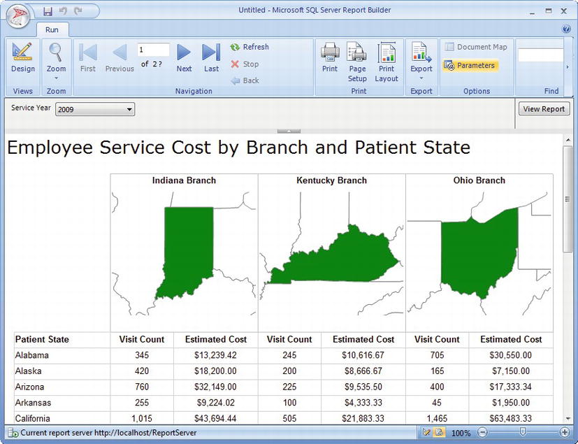
Figure 13-67. Employee Service Cost report by branch and patient state rendered

After running the report, click on one of the branch State maps to drill through to the detail report. If you were to click on Ohio for Service Year 2009, your results would be like those shown in Figure 13-68.

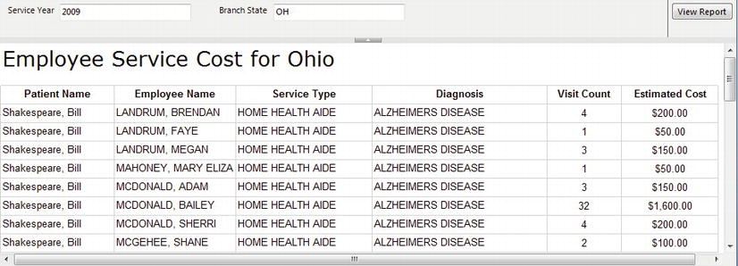
Figure 13-68. Employee Service Cost Detail drill-through report by branch and patient state

Report Parts

There is one more feature that was added with SSRS 2008 R2 that provides some of the true power of ad hoc reporting. As we briefly touched on previously, Report Parts can be created and deployed to the reporting server with the sole purpose of being used by other report developers or ad hoc report authors. Report Parts not only assist in keeping consistency through reusability, but they can also improve report authoring efficiencies. What is also amazing with Report Parts is that when reports consume report parts, if a change is made to the report part, then each report that is using it is notified of the change. The report author can choose to use the new version or keep the existing version that the report is using. This is incredible, I know, and it is a very well received addition to the Report Builder tool.

Before we get into an example, just note that not all report items can be published as report parts. Most of the report items found in the toolbox can be used as a report part, but not all. A list of the report items that can be used are:

• Tablix – Table, List and Matrix
• Charts
• Gauges
• Maps
• Rectangles
• Images
• Parameters

We are going to deploy an existing report to the Report Server as a Report Part. We could do this using the Report Designer or Report Builder, but since we are showing the capabilities of Report Builder 3.0, we will show you how to open up an existing report and deploy it from Report Builder. After we have it deployed, we will show you how report authors using Report Builder 3.0 can “consume” or re-use parts of reports that have been deployed to the Report Server. Open up the Report Builder and let's get started. Here’s what to do:

1. Once you have Report Builder started, click on the Report Builder icon in the top left corner and click Open.
2. Navigate to the location that you have extracted the Pro_SSRS solution and locate the EmployeeSvcCost_RB3_ReportPart.rdl file. Click Open to load the report in Report Builder 3.0.
3. Click Run to view the report to see it in action. The report shows a pie chart with the estimated cost for each branch as shown in Figure 13-69.
   

   Figure 13-69. EmployeeSvcCost_RB3_ReportPart report

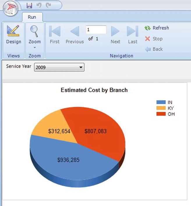
4. Click the Design button to return to design mode. Next, click on the Report Builder menu button again and choose Publish Report Parts, as shown in Figure 13-70.
   

   Figure 13-70. Publish Report Parts

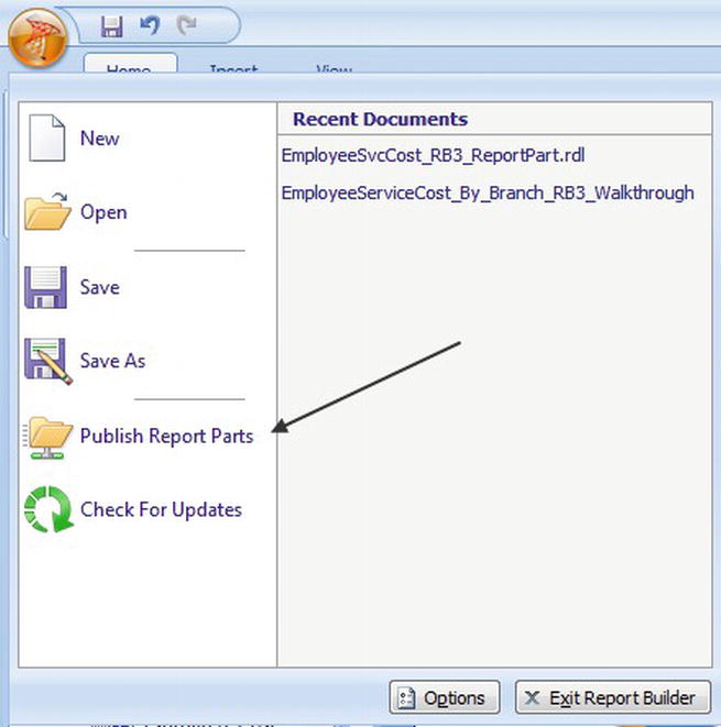
5. On the Publish Report Parts screen, we have the options to Publish all report parts with default settings or to Review and modify report parts before publishing. We could choose the former option, but to show you the ability to deploy individual report items, select the latter option: Review and modify report parts before publishing as depicted in Figure 13-71.
   

   Figure 13-71. Review before publishing

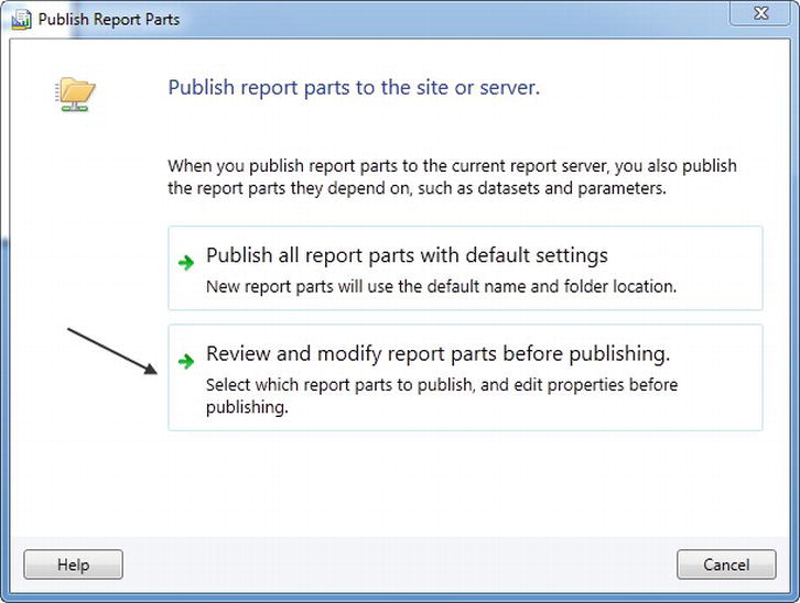
6. As can be seen in Figure 13-72, we have the option to deploy two items in our report. The first being the EstimatedCostByBranch_Pie chart and the second one is our ServiceYear report parameter. Since the Chart needs the parameter, ensure that both are selected and click Publish to deploy our chart to the reporting server.
   

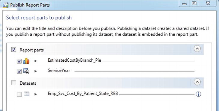
   Figure 13-72. Publish selected report parts

7. If permissions are set appropriately (Content Manager) on the reporting server, you should see two green checkmarks next to the report parts that we had selected to deploy. Click Close to return to Report Builder.
8. Now that we have our report parts deployed, now it is time to create a report that consumes the report part. Click on the Report Builder menu button again and choose New and then choose to create a Blank report. After the new report is loaded change the title of the report to “Estimated Cost by Branch”.
9. Click on the Insert tab in the tabstrip and then select Report Parts. You should see the Report Part Gallery window pane become visible on the right side of the screen, as shown in Figure 13-73. From the Report Part Gallery window, you can search for report parts and see things like what report parts are out there as well as who created them. You can even see what the report part looks like when previewing in thumbnail view.
   

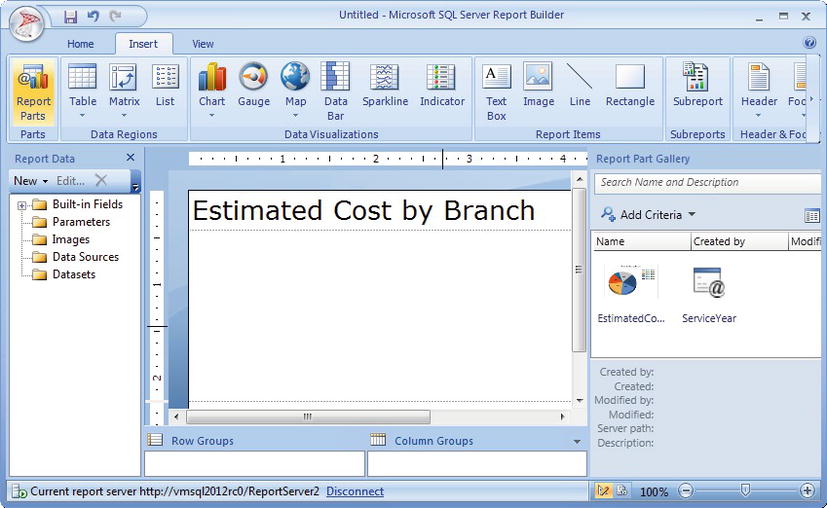
   Figure 13-73. Viewing the report part gallery

10. To use a report part in a report, it is as easy as dragging and dropping the report part onto our design surface. With that being said, drag the EstimatedCostByBranch_Pie chart over onto the design surface and set the left side to be aligned with the header. Click on the home tab and then run the report. Executing the report with ServiceYear 2009 can be seen in Figure 13-74.
11. Save the report to the report server as we did in earlier examples with the name of EstimatedCostByBranch_RB3_Report_Using_ReportPart. We will be looking at this report this later after modifying the report part.

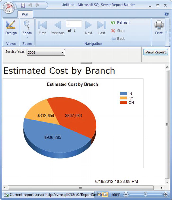
Figure 13-74. Report consuming deployed report part

As you can see, deploying and consuming a report part is a pretty straightforward process. If architected appropriately and some solid report developers, many report parts could be stored on the report server and re-used by report authors to simplify report development.

As you might recall, I mentioned earlier that when changes are made to a report part and it is saved out to the report server, each of the reports that use that report part are then notified of the example. Use the following steps to see this in action:

1. Once you have Report Builder started, click on the Report Builder icon in the top left corner and click Open.
2. Navigate to the location that you have extracted the Pro_SSRS solution and locate the EmployeeSvcCost_RB3_ReportPart.rdl file. Click Open to load the report in Report Builder 3.0. This report is the same report that we opened up earlier. We are now going to make a minor change and then re-publish the report part.
3. Change the font color of the chart title to be Blue and italicized. No major changes, we just want to see what happens when you change a report part. Deploy the report part using the Publish Report Parts as we did earlier from the Report Builder menu button. Only publish the chart this time.
4. Now, let’s go and open the EstimatedCostByBranch_RB3_Report_Using_ReportPart that we saved to the report server which has a copy of the original report part. Click the Report Builder menu button and select Open. Navigate to the report server location where you saved the report and open the EstimatedCostByBranch_RB3_Report_Using_ReportPart report. When you open the report, you should see a message box titled “Updated Report Parts” pop up between the tabstrip and report design surface (Figure 13-75). This is our indicator stating that our report part that we consumed has been altered.
   

   Figure 13-75. Updated report parts message indicator

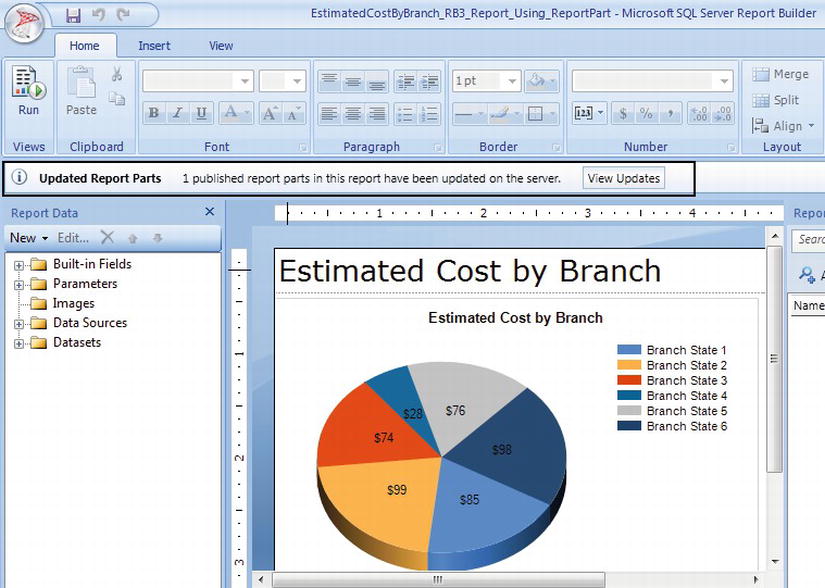
5. Click the View Updates button to see what has changed. When the Update Report Parts screen appears, we should see what has changed as well as a checkbox next to the changed report parts. If we leave the checkbox blank, our report will remain the same as it was and it will not take on these new changes. Conversely, if we place a check in the checkbox, it will update our report with the new report part. We also have the ability to disable the notification when the report part is updated. This essentially tells reporting services that the report doesn’t care if the report part ever changes. If you disable this option, you will not be notified of changes. Click the checkbox to update the EstimatedCostByBranch_Pie report part and click Update as shown in Figure 13-76.

Figure 13-76. Updating reports that consume updated report parts

As you can see by the result of updating our report with the updated report part, we now see a blue, italicized chart title. In my opinion, the Report Part functionality built into Report Builder 3.0 is one of the best additions to ad hoc reporting to date. If you are anything like me, your brain is probably spinning while thinking of new report parts to create for your end users who fall into the report author role —thus, enabling them to quickly and efficiently create ad hoc reports.

Summary

Ad hoc reporting gives users the ability to create their own reports on the fly. It has always been a highly requested feature for any reporting platform and Reporting Services has been no different. As shown in this chapter, Microsoft decided to deliver their first incarnation of ad hoc reporting in the form of Report Builder 1.0. They significantly enhanced the user experience in the Report Builder 2.0 to allow reporting data from relational data and OLAP data sources as well. With the SQL Server 2008 R2 release, came Microsoft’s most recent version, Report Builder 3.0. Furthermore, we showed you an amazing feature called Report Parts that allow report authors to reuse existing sections of reports, saving them hours or potentially days in report development time. In this chapter, you learned about some of their respective benefits and some of their limitations. You have probably come away with an answer to the question of whether the Report Builder is a tool that your users will want. If the answer is “Yes,” as we hope it will be, then the good news is that these are included as standard features.