
Chapter 15. Programmable Pipeline: This Isn’t Your Father’s OpenGL
WHAT YOU’LL LEARN IN THIS CHAPTER:

Graphics hardware has traditionally been designed to quickly perform the same rigid set of hard-coded computations. Different steps of the computation can be skipped, and parameters can be adjusted; but the computations themselves remain fixed. That’s why this old paradigm of GPU design is called fixed functionality.
There has been a trend toward designing general-purpose graphics processors. Just like CPUs, these GPUs can be programmed with arbitrary sequences of instructions to perform virtually any imaginable computation. The biggest difference is that GPUs are tuned for the floating-point operations most common in the world of graphics.
Think of it this way: Fixed functionality is like a cookie recipe. Prior to OpenGL 2.0 you could change the recipe a bit here and there. Change the amount of each ingredient, change the temperature of the oven. You don’t want chocolate chips? Fine. Disable them. But one way or another, you end up with cookies.
Enter programmability with OpenGL 2.0. Want to pick your own ingredients? No problem. Want to cook in a microwave or in a frying pan or on the grill? Have it your way. Instead of cookies, you can bake a cake or grill sirloin or heat up leftovers. The possibilities are endless. The entire kitchen and all its ingredients, appliances, pots, and pans are at your disposal. These are the inputs and outputs, instruction set, and temporary register storage of a programmable pipeline stage.
In this chapter, we cover the conventional OpenGL pipeline and then describe how to replace the programmable portions of it with OpenGL Shading Language shaders.
Out with the Old
Before we talk about replacing it, let’s consider the conventional OpenGL rendering pipeline. The first several stages operate per-vertex. Then the primitive is rasterized to produce fragments. Finally, fragments are textured and fogged, and other per-fragment operations are applied before each fragment is written to the framebuffer. Figure 15.1 diagrams the fixed functionality pipeline.
Figure 15.1. This fixed functionality rendering pipeline represents the old way of doing things.
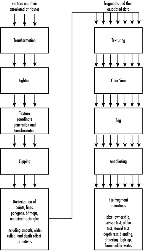
The per-vertex and per-fragment stages of the pipeline are discussed separately in the following sections.
Fixed Vertex Processing
The per-vertex stages start with a set of vertex attributes as input. These attributes include object-space position, normal, primary and secondary colors, and texture coordinates. The final result of per-vertex processing is clip-space position, front-facing and back-facing primary and secondary colors, a fog coordinate, texture coordinates, and point size. What happens in between is broken into four stages, discussed next.
Vertex Transformation
In fixed functionality, the vertex position is transformed from object space to clip space. This is achieved by multiplying the object-space coordinate first by the modelview matrix to put it into eye space. Then it’s multiplied by the projection matrix to reach clip space.
The application has control over the contents of the two matrices, but these matrix multiplications always occur. The only way to “skip” this stage would be to load identity matrices so that you end up with the same position you started with.
Each vertex’s normal is also transformed, this time from object space to eye space for use during lighting. The normal is multiplied by the inverse transpose of the modelview matrix, after which it is optionally rescaled or normalized. Lighting wants the normal to be a unit vector, so unless you’re passing in unit-length normal vectors and have a modelview matrix that leaves them unit length, you’ll need to either rescale them (if your modelview introduced only uniform scaling) or fully normalize them.
Chapter 4, “Geometric Transformations: The Pipeline,” and Chapter 5, “Color, Materials, and Lighting: The Basics,” covered transformations and normals.
Lighting
Lighting takes the vertex color, normal, and position as its raw data inputs. Its output is two colors, primary and secondary, and in some cases a different set of colors for front and back faces. Controlling this stage are the color material properties, light properties, and a variety of glEnable/glDisable toggles.
Lighting is highly configurable; you can enable some number of lights (up to eight or more), each with myriad parameters such as position, color, and type. You can specify material properties to simulate different surface appearances. You also can enable two-sided lighting to generate different colors for front- and back-facing polygons.
You can skip lighting entirely by disabling it. However, when it is enabled, the same hard-coded equations are always used. See Chapter 5, “Color, Materials, and Lighting: The Basics,” and Chapter 6, “More on Color and Materials,” for a refresher on fixed functionality lighting details.
Texture Coordinate Generation and Transformation
The final per-vertex stage of the fixed functionality pipeline involves processing the texture coordinates. Each texture coordinate can optionally be generated automatically by OpenGL. There are several choices of generation equations to use. In fact, a different mode can be chosen for each component of each texture coordinate. Or, if generation is disabled, the current texture coordinate associated with the vertex is used instead.
Whether or not texture generation is enabled, each texture coordinate is always transformed by its texture matrix. If it’s an identity matrix, the texture coordinate is not affected.
This texture coordinate processing stage is covered in Chapter 8, “Texture Mapping: The Basics,” and Chapter 9, “Texture Mapping: Beyond the Basics.”
Clipping
If any of the vertices transformed in the preceding sections happens to fall outside the view volume, clipping must occur. Clipped vertices are discarded, and depending on the type of primitive being drawn, new vertices may be generated at the intersection of the primitive and the view volume. Colors, texture coordinates, and other vertex attributes are assigned to the newly generated vertices by interpolating their values along the clipped edge. Figure 15.2 illustrates a clipped primitive.
Figure 15.2. All three of this triangle’s vertices are clipped out, but six new vertices are introduced.

The application may also enable user clip planes. These clip planes further restrict the clip volume so that even primitives within the view volume can be clipped. This technique is often used in medical imaging to “cut” into a volume of, for example, MRI data to inspect tissues deep within the body.
Fixed Fragment Processing
The per-fragment stages start out with a fragment and its associated data as input. This associated data is comprised of various values interpolated across the line or triangle, including one or more texture coordinates, primary and secondary colors, and a fog coordinate. The result of per-fragment processing is a single color that will be passed along to subsequent per-fragment operations, including depth test and blending. Again, four stages of processing are applied, as covered next.
Texture Application and Environment
Texture application is the most important per-fragment stage. Here, you take all the fragment’s texture coordinates and its primary color as input. The output will be a new primary color. How this happens is influenced by which texture units are enabled for texturing, which texture images are bound to those units, and what texture function is set up by the texture environment.
For each enabled texture unit, the 1D, 2D, 3D, or cube map texture bound to that unit is used as the source for a lookup. Depending on the format of the texture and the texture function specified on that unit, the result of the texture lookup will either replace or be blended with the fragment’s primary color. The resulting color from each enabled texture unit is then fed in as a color input to the next enabled texture unit. The result from the last enabled texture unit is the final output for the texturing stage.
Many configurable parameters affect the texture lookup, including texture coordinate wrap modes, border colors, minification and magnification filters, level-of-detail clamps and biases, depth texture and shadow compare state, and whether mipmap chains are automatically generated. Fixed functionality texturing was covered in detail in Chapters 8 and 9.
Color Sum
The color sum stage starts with two inputs: a primary and a secondary color. The output is a single color. There’s not a lot of magic here. If color sum is enabled, or if lighting is enabled, the primary and secondary colors’ red, green, and blue channels are added together and then clamped back into the range [0,1]. If color sum is not enabled, the primary color is passed through as the result. The alpha channel of the result always comes from the primary color’s alpha. The secondary color’s alpha is never used by the fixed functionality pipeline.
Fog Application
If fog is enabled, the fragment’s color is blended with a constant fog color based on a computed fog factor. That factor is computed according to one of three hard-coded equations: linear, exponential, or second-order exponential. These equations base the fog factor on the current fog coordinate, which may be the approximate distance from the vertex to the eye, or an arbitrary value set per-vertex by the application.
For more details on fixed functionality fog, see Chapter 6.
Antialiasing Application
Finally, if the fragment belongs to a primitive that has smoothing enabled, one piece of associated data is a coverage value. That value is 1.0 in most cases; but for fragments on the edge of a smooth point, line, or polygon, the coverage is somewhere between 0.0 and 1.0. The fragment’s alpha value is multiplied by this coverage value, which, with subsequent blending will produce smooth edges for these primitives. Chapter 6 discusses this behavior.
In with the New
That trip down memory lane was intended to both refresh your memory on the various stages of the current pipeline and give you an appreciation of the configurable but hard-coded computations that happen each step of the way. Now forget everything you just read. We’re going to replace the majority of it and roll in the new world order: shaders.
Shaders are also sometimes called programs, and the terms are usually interchangeable. And that’s what shaders are—application-defined customized programs that take over the responsibilities of fixed functionality pipeline stages. I prefer the term shader because it avoids confusion with the typical definition of program, which can mean any old application.
Figure 15.3 illustrates the simplified pipeline where previously hard-coded stages are subsumed by custom programmable shaders.
Figure 15.3. The block diagram looks simpler, but in reality these shaders can do everything the original fixed stages could do, plus more.

Programmable Vertex Shaders
As suggested by Figure 15.3, the inputs and outputs of a vertex shader remain the same as those of the fixed functionality stages being replaced. The raw vertices and all their attributes are fed into the vertex shader, rather than the fixed transformation stage. Out the other side, the vertex shader spits texture coordinates, colors, point size, and a fog coordinate, which are passed along to the clipper. A vertex shader is a drop-in replacement for the fixed transformation, lighting, and texture coordinate processing per-vertex stages.
Replacing Vertex Transformation
What you do in your vertex shader is entirely up to you. The absolute minimum (if you want anything to draw) would be to output a clip-space vertex position. Every other output is optional and at your sole discretion. How you generate your clip-space vertex position is your call. Traditionally, and to emulate fixed functionality transformation, you would want to multiply your input position by the modelview and projection matrices to get your clip-space output.
But say you have a fixed projection and you’re sending in your vertices already in clip space. In that case, you don’t need to do any transformation. Just copy the input position to the output position. Or, on the other hand, maybe you want to turn your Cartesian coordinates into polar coordinates. You could add extra instructions to your vertex shader to perform those computations.
Replacing Lighting
If you don’t care what the vertex’s colors are, you don’t have to perform any lighting computations. You can just copy the color inputs to the color outputs; or if you know the colors will never be used later, you don’t have to output them at all, and they will become undefined. Beware, if you do try to use them later after not outputting them from the vertex shader, undefined usually means garbage!
If you do want to generate more interesting colors, you have limitless ways of going about it. You could emulate fixed functionality lighting by adding instructions that perform these conventional computations, maybe customizing them here or there. You could also color your vertices based on their positions, their surface normals, or any other input parameter.
Replacing Texture Coordinate Processing
If you don’t need texture coordinate generation, you don’t need to code it into your vertex shader. The same goes for texture coordinate transformation. If you don’t need it, don’t waste precious shader cycles implementing it. You can just copy your input texture coordinates to their output counterparts. Or, as with colors, if you won’t use the texture coordinate later, don’t waste your time outputting it at all. For example, if your GPU supports eight texture coordinates, but you’re going to use only three of them for texturing later in the pipeline, there’s no point in outputting the other five. Doing so would just consume resources unnecessarily.
After reading the preceding sections, you should have a sufficient understanding of the input and output interfaces of vertex shaders; they are largely the same as their fixed functionality counterparts. But there’s been a lot of hand waving about adding code to perform the desired computations within the shader. This would be a great place for an example of a vertex shader, wouldn’t it? Alas, this section covers only the what, where, and why of shaders. The second half of this chapter, and the following two chapters for that matter, are devoted to the how, so you’ll have to be patient and use your imagination. Consider this the calm before the storm. In a few pages, you’ll be staring at more shaders than you ever hoped to see.
Fixed Functionality Glue
In between the vertex shader and the fragment shader, there remain a couple of fixed functionality stages that act as glue between the two shaders. One of them is the clipping stage described previously, which clips the current primitive against the view volume and in so doing possibly adds or removes vertices. After clipping, the perspective divide by W occurs, yielding normalized device coordinates. These coordinates are subjected to viewport transformation and depth range transformation, which yield the final window-space coordinates. Then it’s on to rasterization.
Rasterization is the fixed functionality stage responsible for taking the processed vertices of a primitive and turning them into fragments. Whether a point, line, or polygon primitive, this stage produces the fragments to “fill in” the primitive and interpolates all the colors and texture coordinates so that the appropriate value is assigned to each fragment. Figure 15.4 illustrates this process.
Figure 15.4. Rasterization turns vertices into fragments.
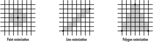
Depending on how far apart the vertices of a primitive are, the ratio of fragments to vertices tends to be relatively high. For a highly tessellated or distant object, though, you might find all three vertices of a triangle mapping to the same single fragment. As a general rule, significantly more fragments than vertices are processed, but as with all rules, there are exceptions.
Rasterization is also responsible for making lines the desired width and points the desired size. It may apply stipple patterns to lines and polygons. It generates partial coverage values at the edges of smooth points, lines, and polygons, which later are multiplied into the fragment’s alpha value during antialiasing application. If requested, rasterization culls out front- or back-facing polygons and applies depth offsets.
In addition to points, lines, and polygons, rasterization also generates the fragments for bitmaps and pixel rectangles (drawn with glDrawPixels). But these primitives don’t originate from normal vertices. Instead, where interpolated data is usually assigned to fragments, those values are adopted from the current raster position. See Chapter 7, “Imaging with OpenGL,” for more details on this subject.
Programmable Fragment Shaders
The same texture coordinates and colors are available to the fragment shader as were previously available to the fixed functionality texturing stage. The same single-color output is expected out of the fragment shader that was previously expected from the fixed functionality fog stage. Just as with vertex shaders, you may choose your own adventure in between the input interface and the output interface.
Replacing Texturing
The single most important capability of a fragment shader is performing texture lookups. For the most part, these texture lookups are unchanged from fixed functionality in that most of the texture state is set up outside the fragment shader. The texture image is specified and all its parameters are set the same as though you weren’t using a fragment shader. The main difference is that you decide within the shader when and whether to perform a lookup and what to use as the texture coordinate.
You’re not limited to using texture coordinate 0 to index into texture image 0. You can mix and match coordinates with different textures, using the same texture with different coordinates or the same coordinate with different textures. Or you can even compute a texture coordinate on the fly within the shader. This flexibility was impossible with fixed functionality.
The texture environment previously included a texture function that determined how the incoming fragment color was mixed with the texture lookup results. That function is now ignored, and it’s up to the shader to combine colors with texture results. In fact, you might choose to perform no texture lookups at all and rely only on other computations to generate the final color result. A fragment shader could simply copy its primary color input to its color output and call it a day. Not very interesting, but such a “passthrough” shader might be all you need when combined with a fancy vertex shader.
Replacing Color Sum
Replacing the color sum is simple. This stage just adds together the primary and secondary colors. If that’s what you want to happen, you just add an instruction to do that. If you’re not using the secondary color for anything, ignore it.
Replacing Fog
Fog application is not as easy to emulate as color sum, but it’s still reasonably easy. First, you need to calculate the fog factor with an equation based on the fragment’s fog coordinate and some constant value such as density. Fixed functionality dictated the use of linear, exponential, or second-order exponential equations, but with shaders you can make up your own equation. Then you blend in a constant fog color with the fragment’s unfogged color, using the fog factor to determine how much of each goes into the blend. You can achieve all this in just a handful of instructions. Or you can not add any instructions and forget about fog. The choice is yours.
OpenGL Shading Language: A First Glimpse
Enough with the hypotheticals. If you’ve made it this far, you must have worked up an appetite for some real shaders by now. Programming GPUs in a high-level language instead of an assembly language means compact and readable code, and thus higher productivity. The OpenGL Shading Language (GLSL) is the name of this language. It looks a lot like C, but with built-in data types and functions that are useful to vertex and fragment shaders.
Listings 15.1 and 15.2 are your first exposure to GLSL shaders. Consider them to be “Hello World” shaders, even though technically they don’t say hello at all.
Listing 15.1. A Simple GLSL Vertex Shader
void main(void)
{
// This is our Hello World vertex shader
// notice how comments are preceded by '//'
// normal MVP transform
vec4 clipCoord = gl_ModelViewProjectionMatrix * gl_Vertex;
gl_Position = clipCoord;
// Copy the primary color
gl_FrontColor = gl_Color;
// Calculate NDC
vec3 ndc = clipCoord.xyz / clipCoord.w;
// Map from [-1,1] to [0,1] before outputting
gl_SecondaryColor = (ndc * 0.5) + 0.5;
}
Listing 15.2. A Simple GLSL Fragment Shader
// This is our Hello World fragment shader
void main(void)
{
// Mix primary and secondary colors, 50/50
gl_FragColor = mix(gl_Color, vec4(vec3(gl_SecondaryColor), 1.0), 0.5);
}
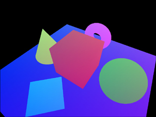
If these shaders are not self-explanatory, don’t despair! The rest of this chapter will make sense of it all. Basically, the vertex shader emulates fixed functionality vertex transformation by multiplying the object-space vertex position by the modelview/projection matrix. Then it copies its primary color unchanged. Finally, it generates a secondary color based on the post-perspective divide normalized device coordinates. Because they will be in the range [–1,1], you also have to divide by 2 and add 0.5 to map colors to the range [0,1]. The fragment shader is left with the simple task of mixing the primary and secondary colors together. Figure 15.5 shows a sample scene rendered with these shaders.
Figure 15.5. Notice how the colors are pastel tinted by the objects’ positions in the scene.
Managing GLSL Shaders
The new GLSL commands are quite a departure from prior core OpenGL API. There’s no more of the Gen/Bind/Delete that you’re used to; GLSL gets all newly styled entry points.
Shader Objects
GLSL uses two types of objects: shader objects and program objects. The first objects we will look at, shader objects, are loaded with shader text and compiled.
Creating and Deleting
You create shader objects by calling glCreateShader and passing it the type of shader you want, either vertex or fragment. This function returns a handle to the shader object used to reference it in subsequent calls:
GLuint myVertexShader = glCreateShader(GL_VERTEX_SHADER);
GLuint myFragmentShader = glCreateShader(GL_FRAGMENT_SHADER);
Beware that object creation may fail, in which case 0 (zero) will be returned. (If this happens, it’s probably due to a simple error in how you called it.) When you’re done with your shader objects, you should clean up after yourself:
glDeleteShader(myVertexShader);
glDeleteShader(myFragmentShader);
Some other OpenGL objects, including texture objects, unbind an object during deletion if it’s currently in use. GLSL objects are different. glDeleteShader simply marks the object for future deletion, which will occur as soon as the object is no longer being used.
Specifying Shader Text
Unlike some other shading language APIs out there, GLSL is designed to accept shader text rather than precompiled binaries. This makes it possible for the application to provide a single universal shader regardless of the underlying OpenGL implementation. The OpenGL device driver can then proceed to compile and optimize for the underlying hardware. Another benefit is that the driver can be updated with improved optimization methods, making shaders run faster over time, without any burden on application vendors to patch their applications.
A shader object’s goal is simply to accept shader text and compile it. Your shader text can be hard-coded as a string-literal, read from a file on disk, or generated on the fly. One way or another, it needs to be in a string so you can load it into your shader object:
GLchar *myStringPtrs[1];
myStringPtrs[0] = vertexShaderText;
glShaderSource(myVertexShader, 1, myStringPtrs, NULL);
myStringPtrs[0] = fragmentShaderText;
glShaderSource(myFragmentShader, 1, myStringPtrs, NULL);
glShaderSource is set up to accept multiple individual strings. The second argument is a count that indicates how many string pointers to look for. The strings are strung together into a single long string before being compiled. This capability can be useful if you’re loading reusable subroutines from a library of functions:
GLchar *myStringPtrs[3];
myStringPtrs[0] = vsMainText;
myStringPtrs[1] = myNoiseFuncText;
myStringPtrs[2] = myBlendFuncText;
glShaderSource(myVertexShader, 3, myStringPtrs, NULL);
If all your strings are null-terminated, you don’t need to specify string lengths in the fourth argument and can pass in NULL instead. But for shader text that is not null-terminated, you need to provide the length; lengths do not include the null terminator if present. You can use –1 for strings that are null-terminated. The following code passes in a pointer to an array of lengths along with the array of string pointers:
GLint fsLength = strlen(fragmentShaderText);
myStringPtrs[0] = fragmentShaderText;
glShaderSource(myFragmentShader, 1, myStringPtrs, &fsLength);
Compiling Shaders
After your shader text is loaded into a shader object, you need to compile it. Compiling parses your shader and makes sure there are no errors:
glCompileShader(myVertexShader);
glCompileShader(myFragmentShader);
You can query a flag in each shader object to see whether the compile was successful. Each shader object also has an information log that contains error messages if the compilation failed. It might also contain warnings or other useful information even if your compilation was successful. These logs are primarily intended for use as a tool while you are developing your GLSL application:
glCompileShader(myVertexShader);
glGetShaderiv(myVertexShader, GL_COMPILE_STATUS, &success);
if (!success)
{
GLchar infoLog[MAX_INFO_LOG_SIZE];
glGetShaderInfoLog(myVertexShader, MAX_INFO_LOG_SIZE, NULL, infoLog);
fprintf(stderr, "Error in vertex shader compilation!
");
fprintf(stderr, "Info log: %s
", infoLog);
}
The returned info log string is always null-terminated. If you don’t want to allocate a large static array to store the info log, you can find out the exact size of the info log before querying it:
glGetShaderiv(myVertexShader, GL_INFO_LOG_LENGTH, &infoLogSize);
Program Objects
The second type of object GLSL uses is a program object. This object acts as a container for shader objects, linking them together into a single executable. You can specify a GLSL shader for each replaceable section of the conventional OpenGL pipeline. Currently, only vertex and fragment stages are replaceable, but that list could be extended in the future to include additional stages.
Creating and Deleting
Program objects are created and deleted the same way as shader objects. The difference is that there’s only one kind of program object, so its creation command doesn’t take an argument:
GLuint myProgram = glCreateProgram();
...
glDeleteProgram(myProgram);
Attaching and Detaching
A program object is a container. You need to attach your shader objects to it if you want GLSL instead of fixed functionality:
glAttachShader(myProgram, myVertexShader);
glAttachShader(myProgram, myFragmentShader);
You can even attach multiple shader objects of the same type to your program object. Similar to loading multiple shader source strings into a single shader object, this makes it possible to include function libraries shared by more than one of your program objects.
You can choose to replace only part of the pipeline with GLSL and leave the rest to fixed functionality. Just don’t attach shaders for the parts you want to leave alone. Or if you’re switching between GLSL and fixed functionality for part of the pipeline, you can detach a previously attached shader object. You can even detach both shaders, in which case you’re back to full fixed functionality:
glDetachShader(myProgram, myVertexShader);
glDetachShader(myProgram, myFragmentShader);
Linking Programs
Before you can use GLSL for rendering, you have to link your program object. This process takes each of the previously compiled shader objects and links them into a single executable:
glLinkProgram(myProgram);
You can query a flag in the program object to see whether the link was successful. The object also has an information log that contains error messages if the link failed. The log might also contain warnings or other useful information even if your link was successful:
glLinkProgram(myProgram);
glGetProgramiv(myProgram, GL_LINK_STATUS, &success);
if (!success)
{
GLchar infoLog[MAX_INFO_LOG_SIZE];
glGetProgramInfoLog(myProgram, MAX_INFO_LOG_SIZE, NULL, infoLog);
fprintf(stderr, "Error in program linkage!
");
fprintf(stderr, "Info log: %s
", infoLog);
}
Validating Programs
If your link was successful, odds are good that your shaders will be executable when it comes time to render. But some things aren’t known at link time, such as the values assigned to texture samplers, described in subsequent sections. A sampler may be set to an invalid value, or multiple samplers of different types may be illegally set to the same value. At link time, you don’t know what the state is going to be when you render, so errors cannot be thrown at that time. When you validate, however, it looks at the current state so you can find out once and for all whether your GLSL shaders are going to execute when you draw that first triangle:
glValidateProgram(myProgram);
glGetProgramiv(myProgram, GL_VALIDATE_STATUS, &success);
if (!success)
{
GLchar infoLog[MAX_INFO_LOG_SIZE];
glGetProgramInfoLog(myProgram, MAX_INFO_LOG_SIZE, NULL, infoLog);
fprintf(stderr, "Error in program validation!
");
fprintf(stderr, "Info log: %s
", infoLog);
}
Again, if the validation fails, an explanation and possibly tips for avoiding the failure are included in the program object’s info log. Note that validating your program object before rendering with it is not a requirement, but if you do try to use a program object that would have failed validation, your rendering commands will fail and throw OpenGL errors.
Using Programs
Finally, you’re ready to turn on your program. Unlike other OpenGL features, GLSL mode is not toggled with glEnable/glDisable. Instead, use this:
glUseProgram(myProgram);
You can use this function to enable GLSL with a particular program object and also to switch between different program objects. To disable GLSL and switch back to fixed functionality, you also use this function, passing in 0:
glUseProgram(0);
You can query for the current program object handle at any time:
currentProgObj = glGetIntegerv(GL_CURRENT_PROGRAM);
Now that you know how to manage your shaders, you can focus on their contents. The syntax of GLSL is largely the same as that of C/C++, so you should be able to dive right in. It should be noted that the latest version of the GLSL specification at the time of publishing is v1.20.
Variables
Variables and functions must be declared in advance. Your variable name can use any letters (case-sensitive), numbers, or an underscore, but it can’t begin with a number. Also, your variable cannot begin with the prefix gl_, which is reserved for built-in variables and functions. A list of reserved keywords available in the OpenGL Shading Language specification contains a list of reserved keywords, which are also off-limits.
Basic Types
In addition to the Boolean, integer, and floating-point types found in C, GLSL introduces some data types commonly used in shaders. Table 15.1 lists these basic data types.

Structures
Structures can be used to group basic data types into a user-defined data type. When defining the structure, you can declare instances of the structure at the same time, or you can declare them later:
struct surface {
float indexOfRefraction;
float reflectivity;
vec3 color;
float turbulence;
} myFirstSurf;
surface mySecondSurf;
You can assign one structure to another (=) or compare two structures (==, !=). For both of these operations, the structures must be of the same declared type. Two structures are considered equal if each of their member fields is component-wise equal. To access a single field of a structure, you use the selector (.):
vec3 totalColor = myFirstSurf.color + mySecondSurf.color;
Structure definitions must contain at least one member. Arrays, discussed next, may be included in structures, but only when a specific array size is provided. Unlike C language structures, GLSL does not allow bit fields. Structures within structures are also not allowed.
struct superSurface {
vec3 points[30]; // Sized arrays are okay
surface surf; // Okay, as surface was defined earlier
struct velocity { // ILLEGAL!! Embedded struct
float speed;
vec3 direction;
} velo;
subSurface sub; // ILLEGAL!! Forward declaration
};
struct subSurface {
int id;
};
Arrays
One-dimensional arrays of any type (including structures) can be declared. You don’t need to declare the size of the array as long as it is always indexed with a constant integer expression. Otherwise, you must declare its size up front. All the following are acceptable:
surface mySurfaces[];
vec4 lightPositions[8];
vec4 moreLightPositions[] = lightPositions;
const int numSurfaces = 5;
surface myFiveSurfaces[numSurfaces];
float[5] values; // another way to size the array
You also must declare an explicit size for your array when the array is declared as a parameter or return type in a function declaration or as a member of a structure.
The length() method can be used to return the length of an array:
lightPositions.length(); // returns array size, in this case 8
One last thing: You cannot declare an array of arrays!
Qualifiers
Variables can be declared with an optional type qualifier. Table 15.2 lists the available qualifiers.

Built-In Variables
Built-in variables allow interaction with fixed functionality. They don’t need to be declared before use. Tables 15.3 and 15.4 list most of the built-in variables. Refer to the GLSL specification for built-in uniforms and constants.
Table 15.3. Built-in Vertex Shader Variables
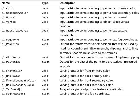
Table 15.4. Built-in Fragment Shader Variables

Expressions
The following sections describe various operators and expressions found in GLSL.
Operators
All the familiar C operators are available in GLSL with few exceptions. See Table 15.5 for a complete list.
Table 15.5. Operators in Order of Precedence (From Highest to Lowest)

A few operators are missing from GLSL. Because there are no pointers to worry about, you don’t need an address-of operator (&) or a dereference operator (*). A typecast operator is not needed because typecasting is not allowed. Bitwise operators (&, |, ^, ~, <<, >>, &=, |=, ^=, <<=, >>=) are reserved for future use, as are modulus operators (%, %=).
Array Access
Arrays are indexed using integer expressions, with the first array element at index 0:
vec4 myFifthColor, ambient, diffuse[6], specular[6];
...
myFifthColor = ambient + diffuse[5] + specular[5];
Shader execution is undefined if an attempt is made to access an array with an index less than zero or greater than or equal to the size of the array. If the compiler can determine this at compile time (e.g., the array is indexed by an out-of-range constant expression), the shader will fail to compile entirely.
Constructors
Constructors are special functions primarily used to initialize variables, especially of multicomponent data types, including structures and arrays. They take the form of a function call with the name of the function being the same as the name of the type:
vec3 myNormal = vec3(0.0, 1.0, 0.0);
Constructors are not limited to declaration initializers; they can be used as expressions anywhere in your shader:
greenTint = myColor + vec3(0.0, 1.0, 0.0);
A single scalar value is assigned to all elements of a vector:
ivec4 myColor = ivec4(255); // all 4 components get 255
You can mix and match scalars, vectors, and matrices in your constructor, as long as you end up with enough components to initialize the entire data type. Any extra components are dropped:
vec4 myVector1 = vec4(x, vec2(y, z), w);
vec2 myVector2 = vec2(myVector1); // z, w are dropped
float myFloat = float(myVector2); // y dropped
Matrices are constructed in column-major order. If you provide a single scalar value, that value is used for the diagonal matrix elements, and all other elements are set to 0:
// all of these are same 2x2 identity matrix
mat2 myMatrix1 = mat2(1.0, 0.0, 0.0, 1.0);
mat2 myMatrix2 = mat2(vec2(1.0, 0.0), vec2(0.0, 1.0));
mat2 myMatrix3 = mat2(1.0);
mat2 myMatrix4 = mat2(mat4(1.0)); // takes upper 2x2 of the 4x4
You can also use constructors to convert between the different scalar types. This is the only way to perform type conversions. No implicit or explicit typecasts or promotions are possible.
The conversion from int to float is obvious. When you are converting from float to int, the fractional part is dropped. When you are converting from int or float to bool, values of 0 or 0.0 are converted to false, and anything else is converted to true. When you are converting from bool to int or float, true is converted to 1 or 1.0, and false is converted to 0 or 0.0:
float myFloat = 4.7;
int myInt = int(myFloat); // myInt = 4
Arrays can be initialized by providing in the constructor a value for every element of the array. Either of the following is acceptable:
ivec2 cursorPositions[3] = ivec2[3]((0, 0), (10, 20), (15, 40));
ivec2 morePositions[3] = ivec2[]((0, 0), (10, 20), (15, 40));
Finally, you can initialize structures by providing arguments in the same order and of the same type as the structure definition:
struct surface {
float indexOfRefraction;
float reflectivity;
vec3 color;
float turbulence;
};
surface mySurf = surface(ior, refl, vec3(red, green, blue), turb);
Component Selectors
Individual components of a vector can be accessed by using dot notation along with {x,y,z,w}, {r,g,b,a}, or {s,t,p,q}. These different notations are useful for positions and normals, colors, and texture coordinates, respectively. You cannot mix and match selectors from the different notations. Notice the p in place of the usual r texture coordinate. This component has been renamed to avoid ambiguity with the r color component. Here are some examples of component selectors:
vec3 myVector = {0.25, 0.5, 0.75};
float myR = myVector.r; // 0.25
vec2 myYZ = myVector.yz; // 0.5, 0.75
float myQ = myVector.q; // ILLEGAL!! accesses component beyond vec3
float myRY = myVector.ry; // ILLEGAL!! mixes two notations
You can use the component selectors to rearrange the order of components or replicate them:
vec3 myZYX = myVector.zyx; // reverse order
vec4 mySSTT = myVector.sstt; // replicate s and t twice each
You can also use them as write masks on the left side of an assignment to select which components are modified. In this case, you cannot use component selectors more than once:
vec4 myColor = vec4(0.0, 1.0, 2.0, 3.0);
myColor.x = -1.0; // -1.0, 1.0, 2.0, 3.0
myColor.yz = vec2(-2.0, -3.0); // -1.0, -2.0, -3.0, 3.0
myColor.wx = vec2(0.0, 1.0); // 1.0, -2.0, -3.0, 0.0
myColor.zz = vec2(2.0, 3.0); // ILLEGAL!!
Another way to get at individual vector components or matrix components is to use array subscript notation. This way, you can use an arbitrarily computed integer index to access your vector or matrix as if it were an array. Shader execution is undefined if an attempt is made to access a component outside the bounds of the vector or matrix.
float myY = myVector[1];
For matrices, providing a single array index accesses the corresponding matrix column as a vector. Providing a second array index accesses the corresponding vector component:
mat3 myMatrix = mat3(1.0);
vec3 myFirstColumn = myMatrix[0]; // first column: 1.0, 0.0, 0.0
float element21 = myMatrix[2][1]; // last column, middle row: 0.0
Control Flow
GLSL offers a variety of familiar nonlinear flow mechanisms that reduce code size, make more complex algorithms possible, and make shaders more readable.
Loops
for, while, and do/while loops are all supported with the same syntax as in C/C++. Loops can be nested. You can use continue and break to prematurely move on to the next iteration or break out of the loop:
for (l = 0; l < numLights; l++)
{
if (!lightExists[l])
continue;
color += light[l];
}
while (lightNum >= 0)
{
color += light[lightNum];
lightNum—;
}
do
{
color += light[lightNum];
lightNum—;
} while (lightNum > 0);
if/else
You can use if and if/else clauses to select between multiple blocks of code. These conditionals can also be nested:
color = unlitColor;
if (numLights > 0)
{
color = litColor;
}
if (numLights > 0)
{
color = litColor;
}
else
{
color = unlitColor;
}
discard
Fragment shaders have a special control flow mechanism called discard. It terminates execution of the current fragment’s shader. All subsequent per-fragment pipeline stages are skipped, and the fragment is not written to the framebuffer:
// e.g., perform an alpha test within your fragment shader
if (color.a < 0.9)
discard;
Functions
Functions are used to modularize shader code. All shaders must define a main function, which is the place where execution begins. The void parameter list here is optional, but not the void return:
void main(void)
{
...
}
Functions must be either defined or declared with a prototype before use. These definitions or declarations should occur globally, outside any function. Return types are required, as are types for each function argument. Also, arguments can have an optional qualifier in, out, inout, or const (see Table 15.2):
// function declaration
bool isAnyComponentNegative(const vec4 v);
// function use
void main()
{
bool someNeg = isAnyComponentNegative(gl_MultiTexCoord0);
...
}
// function definition
bool isAnyComponentNegative(const vec4 v)
{
if ((v.x < 0.0) || (v.y < 0.0) ||
(v.z < 0.0) || (v.w < 0.0))
return true;
else
return false;
}
Structures are allowed as arguments and return types. Arrays are also allowed as arguments and return types, in which case the declaration and definition would include the array name with size, whereas the function call would just use the array name without brackets or size:
vec4 sumMyVectors(int howManyToSum, vec4 v[10]);
void main()
{
vec4 myColors[10];
...
gl_FragColor = sumMyVectors(6, myColors);
}
You can give more than one function the same name, as long as the return type or argument types are different. This is called function name overloading and is useful if you want to perform the same type of operation on, for example, different-sized vectors:
float multiplyAccumulate(float a, float b, float c)
{
return (a * b) + c; // scalar definition
}
vec4 multiplyAccumulate(vec4 a, vec4 b, vec4 c)
{
return (a * b) + c; // 4-vector definition
}
Recursive functions are not allowed. In other words, the same function cannot be present more than once in the current call stack. Some compilers may be able to catch this and throw an error, but in any case, shader execution will be undefined.
Approximately 50 built-in functions provide all sorts of useful calculations, ranging from simple arithmetic to trigonometry. You can consult the GLSL specification for the complete list and descriptions.
Texture Lookup Functions
Texture lookup built-in functions deserve special mention. Whereas some of the other built-in functions are provided as a convenience because you could code your own versions relatively easily, texture lookup built-in functions (shown in the following list) are crucial to perform even the most basic texturing.
Texture Lookup Built-in Functions
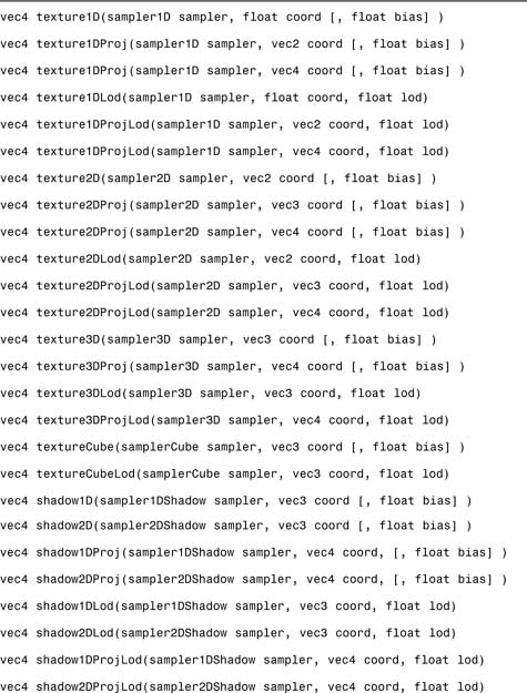
The lookup is performed on the texture of the type encoded in the function name (1D, 2D, 3D, Cube) currently bound to the sampler represented by the sampler parameter. The “Proj” versions perform a perspective divide on the texture coordinate before lookup. The divisor is the last component of the coordinate vector.
The “Lod” versions, available only in a vertex shader, specify the mipmap level-of-detail (LOD) from which to sample. The non-“Lod” versions sample from the base LOD when used by a vertex shader. Fragment shaders can use only the non-“Lod” versions, where the mipmap LOD is computed as usual based on texture coordinate derivatives. However, fragment shaders can supply an optional bias that will be added to the computed LOD. This bias parameter is not allowed in a vertex shader.
The “shadow” versions perform a depth texture comparison as part of the lookup (see Chapter 14, “Depth Textures and Shadows”).
Summary
In this chapter, we outlined the conventional per-vertex and per-fragment pipeline stages, setting the stage for their wholesale replacement by programmable stages. You learned all the nuts and bolts of the OpenGL Shading Language (GLSL). We discussed all the variable types, operators, and flow control mechanisms. We also described how to use the commands for loading and compiling shader objects and linking and using program objects. There was a lot of ground to cover here, but we made it through at a record pace.
This concludes the boring lecture portion of our shader coverage. You now have a solid conceptual foundation for the next two chapters, which will provide practical examples of vertex and fragment shader applications using GLSL. The following chapters will prove much more enjoyable with all the textbook learning behind you.