
Chapter 16. Vertex Shading: Do-It-Yourself Transform, Lighting, and Texgen
WHAT YOU’LL LEARN IN THIS CHAPTER:
• How to perform per-vertex lighting
• How to generate texture coordinates
• How to calculate per-vertex fog
• How to calculate per-vertex point size
• How to squash and stretch objects
• How to make realistic skin with vertex blending
This chapter is devoted to the application of vertex shaders. We covered the basic mechanics of OpenGL Shading Language (GLSL) shaders in the preceding chapter, but at some point you have to put the textbook down and start learning by doing. Here, we introduce a handful of shaders that perform various real-world tasks. You are encouraged to use these shaders as a starting point for your own experimentation.
Getting Your Feet Wet
Every shader should at the very least output a clip-space vertex coordinate. Lighting and texture coordinate generation (texgen), the other operations typically performed in vertex shaders, may not be necessary. For example, if you’re creating a depth texture and all you care about are the final depth values, you wouldn’t waste instructions in your shader to output a color or texture coordinates. But one way or another, you always need to output a clip-space position for subsequent primitive assembly and rasterization to occur.
For your first sample shader, you’ll perform the bare-bones vertex transformation that would occur automatically by fixed functionality if you weren’t using a vertex shader. As an added bonus, you’ll copy the incoming color into the outgoing color. Remember, anything that isn’t output remains undefined. If you want that color to be available later in the pipeline, you have to copy it from input to output, even if the vertex shader doesn’t need to change it in any way.
Figure 16.1 shows the result of the simple shader in Listing 16.1.
Figure 16.1. This vertex shader transforms the position to clip space and copies the vertex’s color from input to output.
Listing 16.1. Simple Vertex Shader
// simple.vs
//
// Generic vertex transformation,
// copy primary color
void main(void)
{
// multiply object-space position by MVP matrix
gl_Position = gl_ModelViewProjectionMatrix * gl_Vertex;
// Copy the primary color
gl_FrontColor = gl_Color;
}
The modelview and projection matrices are traditionally two separate matrices against which the incoming object-space vertex position is multiplied. GLSL conveniently provides a shortcut called gl_ModelViewProjectionMatrix, a concatenation of the two matrices, which we refer to as the MVP matrix. This way we need only perform one matrix multiply in order to transform the vertex position.
An alternative to performing the transform yourself is using the ftransform built-in function, which emulates fixed functionality vertex transformation on the incoming vertex position. Not only is it convenient, but it also guarantees that the result is identical to that achieved by fixed functionality, which is especially useful when rendering in multiple passes. Otherwise, if you mix fixed functionality and your own vertex shader (without ftransform) and draw the same geometry, the subtle floating-point differences in the resulting Z values may result in “Z-fighting” artifacts. The invariant qualifier, described in Chapter 15, “Programmable Pipeline: This Isn’t Your Father’s OpenGL,” can be used when declaring vertex shader outputs to achieve a similar effect. Unlike ftransform, however, invariant is not limited to clip-space position.
Diffuse Lighting
Diffuse lighting takes into account the orientation of a surface relative to the direction of incoming light. The following is the equation for diffuse lighting:
Cdiff = max{N • L, 0} * Cmat * Cli
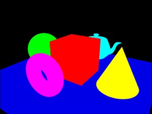
N is the vertex’s unit normal, and L is the unit vector representing the direction from the vertex to the light source. Cmat is the color of the surface material, and Cli is the color of the light. Cdiff is the resulting diffuse color. Because the light in the example is white, you can omit that term, as it would be the same as multiplying by {1,1,1,1}. Figure 16.2 shows the result from Listing 16.2, which implements the diffuse lighting equation.
Figure 16.2. This vertex shader computes diffuse lighting. (This figure also appears in the Color insert.)

Listing 16.2. Diffuse Lighting Vertex Shader
// diffuse.vs
//
// Generic vertex transformation,
// diffuse lighting based on one
// white light
uniform vec3 lightPos[1];
void main(void)
{
// normal MVP transform
gl_Position = gl_ModelViewProjectionMatrix * gl_Vertex;
vec3 N = normalize(gl_NormalMatrix * gl_Normal);
vec4 V = gl_ModelViewMatrix * gl_Vertex;
vec3 L = normalize(lightPos[0] - V.xyz);
// output the diffuse color
float NdotL = dot(N, L);
gl_FrontColor = gl_Color * vec4(max(0.0, NdotL));
}
The light position is a uniform vector passed into the shader from the application. This allows you to easily change the light position interactively without having to alter the shader. You can do this using the left- and right-arrow keys while running the VertexShaders sample program. It could have been referenced instead using the built-in uniform variable gl_LightSource[n].position to achieve the same effect, in which case the sample program would call glLight* instead of glUniform* to update the position.
After computing the clip-space position as you did in the “simple” shader, the “diffuse” shader proceeds to transform the vertex position to eye space, too. All the lighting calculations are performed in eye space, so you need to transform the normal vector from object space to eye space as well. GLSL provides the gl_NormalMatrix built-in uniform matrix as a convenience for this purpose. It is simply the inverse transpose of the modelview matrix’s upper-left 3×3 elements. The last vector you need to compute is the light vector, which is the direction from the vertex position to the light position, so you just subtract one from the other. Note that we’re modeling a point light here rather than a directional light.
Both the normal and the light vectors must be unit vectors, so you normalize them before continuing. GLSL supplies a built-in function, normalize, to perform this common task.
The dot product of the two unit vectors, N and L, will be in the range [–1,1]. But because you’re interested in the amount of diffuse lighting bouncing off the surface, having a negative contribution doesn’t make sense. This is why you clamp the result of the dot product to the range [0,1] by using the max function. The diffuse lighting contribution can then be multiplied by the vertex’s diffuse material color to obtain the final lit color.
Specular Lighting
Specular lighting takes into account the orientation of a surface relative to both the direction of incoming light and the view vector. The following is the equation for specular lighting:
Cspec = max{N • H, 0}Sexp * Cmat * Cli
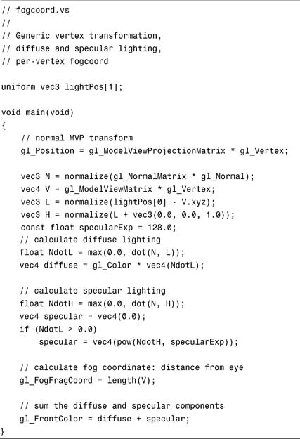
H is the unit vector representing the direction halfway between the light vector and the view vector, known as the half-angle vector. Sexp is the specular exponent, controlling the tightness of the specular highlight. Cspec is the resulting specular color. N, L, Cmat, and Cli represent the same values as in diffuse lighting, although you’re free to use different specular and diffuse colors. Because the light in the example is white, you can again omit that term. Figure 16.3 illustrates the output of Listing 16.3, which implements both diffuse and specular lighting equations. Note that the specular term is included only when N • L is also greater than zero—a subtlety not captured in the above equation, but one that’s part of the fixed functionality lighting definition.
Figure 16.3. This vertex shader computes diffuse and specular lighting. (This figure also appears in the Color insert.)

Listing 16.3. Diffuse and Specular Lighting Vertex Shader

We used a hard-coded constant specular exponent of 128, which provides a nice, tight specular highlight. You can experiment with different values to find one you may prefer. Practice your GLSL skills by turning this scalar value into another uniform that you can control from the application.
Improved Specular Lighting
Specular highlights change rapidly over the surface of an object. Trying to compute them per-vertex and then interpolating the result across a triangle gives relatively poor results. Instead of a nice circular highlight, you end up with a muddy polygonal-shaped highlight.
One way you can improve the situation is to separate the diffuse lighting result from the specular lighting result, outputting one as the vertex’s primary color and the other as the secondary color. By adding the diffuse and specular colors together, you effectively saturate the color (that is, exceed a value of 1.0) wherever a specular highlight appears. If you try to interpolate the sum of these colors, the saturation will more broadly affect the entire triangle. However, if you interpolate the two colors separately and then sum them per-fragment, the saturation will occur only where desired, cleaning up some of the muddiness. When using fixed functionality fragment processing, this sum per-fragment is achieved by simply enabling GL_COLOR_SUM. Here is the altered shader code for separating the two lit colors:
// put diffuse into primary color
float NdotL = max(0.0, dot(N, L));
gl_FrontColor = gl_Color * vec4(NdotL);
// put specular into secondary color
float NdotH = max(0.0, dot(N, H));
gl_FrontSecondaryColor = (NdotL > 0.0) ?
vec4(pow(NdotH, specularExp)) :
vec4(0.0);
Separating the colors improves things a bit, but the root of the problem is the specular exponent. By raising the specular coefficient to a power, you have a value that wants to change much more rapidly than per-vertex interpolation allows. In fact, if your geometry is not tessellated finely enough, you may lose a specular highlight altogether.
An effective way to avoid this problem is to output just the specular coefficient (N • H), but wait and raise it to a power per-fragment. This way, you can safely interpolate the more slowly changing (N • H). You’re not employing fragment shaders until the next chapter, so how do you perform this power computation per-fragment? All you have to do is set up a 1D texture with a table of s128 values and send (N • H) out of the vertex shader on a texture coordinate. This is considered custom texgen. Then you will use fixed functionality texture environment to add the specular color from the texture lookup to the interpolated diffuse color from the vertex shader.
The following is the shader code, again altered from the original specular lighting shader:
// put diffuse lighting result in primary color
float NdotL = max(0.0, dot(N, L));
gl_FrontColor = gl_Color * vec4(NdotL);
// copy (N.H)*8-7 into texcoord if N.L is positive
float NdotH = 0.0;
if (NdotL > 0.0)
NdotH = max(0.0, dot(N, H) * 8.0 - 7.0);
gl_TexCoord[0] = vec4(NdotH, 0.0, 0.0, 1.0);
Here, the (N • H) has been clamped to the range [0,1]. But if you try raising most of that range to the power of 128, you’ll get results so close to zero that they will correspond to texel values of zero. Only the upper 1/8 of (N • H) values will begin mapping to measurable texel values. To make economical use of the 1D texture, you can focus in on this upper 1/8 and fill the entire texture with values from this range, improving the resulting precision. This requires that you scale (N • H) by 8 and bias by –7 so that [0,1] maps to [–7,1]. By using the GL_CLAMP_TO_EDGE wrap mode, values in the range [–7,0] will be clamped to 0. Values in the range of interest, [0,1], will receive texel values between (7/8)128 and 1.
The specular contribution resulting from the texture lookup is added to the diffuse color output from the vertex shader using the GL_ADD texture environment function.
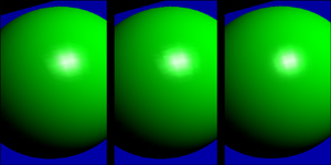
Figure 16.4 compares the three specular shaders to show the differences in quality. An even more precise method would be to output only the normal vector from the vertex shader and to encode a cube map texture so that at every N coordinate the resulting texel value is (N • H)128. We’ve left this as another exercise for you.
Figure 16.4. The per-vertex specular highlight is improved by using separate specular or a specular exponent texture. (This figure also appears in the Color insert.)
Now that you have a decent specular highlight, you can get a little fancier and take the one white light and replicate it into three colored lights. This activity involves performing the same computations, except now you have three different light positions and you have to take the light color into consideration.
As has been the case with all the lighting shaders, you can change the light positions in the sample by using the left- and right-arrow keys. Figure 16.5 shows the three lights in action, produced by Listing 16.4.
Figure 16.5. Three lights are better than one. (This figure also appears in the Color insert.)

Listing 16.4. Three Colored Lights Vertex Shader


Interesting to note in this sample is the use of a loop construct. Even though GLSL permits them, some older OpenGL implementations may not support loops in hardware. So if your shader is running really slowly, it may be emulating the shader execution in software. “Unrolling” the loop—that is, replicating the code within the loop multiple times into a long linear sequence—could alleviate the problem, but at the expense of making your code less readable.
Per-Vertex Fog
Though fog is specified as a per-fragment rasterization stage that follows texturing, often implementations perform most of the necessary computation per-vertex and then interpolate the results across the primitive. This shortcut is sanctioned by the OpenGL specification because it improves performance with very little loss of image fidelity. The following is the equation for a second-order exponential fog factor, which controls the blending between the fog color and the unfogged fragment color:
ff = e–(d*fc)2
In this equation, ff is the computed fog factor. d is the density constant that controls the “thickness” of the fog. fc is the fog coordinate, which is usually the distance from the vertex to the eye, or is approximated by the absolute value of the vertex position’s Z component in eye space. In this chapter’s sample shaders, you’ll compute the actual distance.
In the first sample fog shader, you’ll compute only the fog coordinate and leave it to fixed functionality to compute the fog factor and perform the blend. In the second sample, you’ll compute the fog factor yourself within the vertex shader and also perform the blending per-vertex. Performing all these operations per-vertex instead of per-fragment is more efficient and provides acceptable results for most uses. Figure 16.6 illustrates the fogged scene, which is nearly identical for the two sample fog shaders, the first of which is shown in Listing 16.5.
Figure 16.6. Applying per-vertex fog using a vertex shader. (This figure also appears in the Color insert.)

Listing 16.5. Fog Coordinate Generating Vertex Shader
The calculation to find the distance from the eye (0,0,0,1) to the vertex in eye space is trivial. You need only call the built-in length() function, passing in the vertex position vector as an argument.
The following is the altered GLSL code for performing the fog blend within the shader instead of in fixed functionality fragment processing:
uniform float density;
...
// calculate 2nd order exponential fog factor
const float e = 2.71828;
float fogFactor = (density * length(V));
fogFactor *= fogFactor;
fogFactor = clamp(pow(e, -fogFactor), 0.0, 1.0);
// sum the diffuse and specular components, then
// blend with the fog color based on fog factor
const vec4 fogColor = vec4(0.5, 0.8, 0.5, 1.0);
gl_FrontColor = mix(fogColor, clamp(diffuse + specular, 0.0, 1.0),
fogFactor);
Per-Vertex Point Size
Applying fog attenuates object colors the farther away they are from the viewpoint. Similarly, you can attenuate point sizes so that points rendered close to the viewpoint are relatively large and points farther away diminish into nothing. Like fog, point attenuation is a useful visual cue for conveying perspective. The computation required is similar as well.
You compute the distance from the vertex to the eye exactly the same as you did for the fog coordinate. Then, to get a point size that falls off exponentially with distance, you square the distance, take its reciprocal, and multiply it by the constant 100,000. This constant is chosen specifically for this scene’s geometry so that objects toward the back of the scene, as rendered from the initial camera position, are assigned point sizes of approximately 1, whereas points near the front are assigned point sizes of approximately 10.
In this sample application, you’ll set the polygon mode for front- and back-facing polygons to GL_POINT so that all the objects in the scene are drawn with points. Also, you must enable GL_VERTEX_PROGRAM_POINT_SIZE_ARB so that the point sizes output from the vertex shader are substituted in place of the usual OpenGL point size. Figure 16.7 shows the result of Listing 16.6.
Figure 16.7. Per-vertex point size makes distant points smaller. (This figure also appears in the Color insert.)

Listing 16.6. Point Size Generating Vertex Shader
// ptsize.vs
//
// Generic vertex transformation,
// attenuated point size
void main(void)
{
// normal MVP transform
gl_Position = gl_ModelViewProjectionMatrix * gl_Vertex;
vec4 V = gl_ModelViewMatrix * gl_Vertex;
gl_FrontColor = gl_Color;
// calculate point size based on distance from eye
float ptSize = length(V);
ptSize *= ptSize;
gl_PointSize = 100000.0 / ptSize;
}
Customized Vertex Transformation
You’ve already customized lighting, texture coordinate generation, and fog coordinate generation. But what about the vertex positions themselves? The next sample shader applies an additional transformation before transforming by the usual modelview/projection matrix.
Figure 16.8 shows the effects of scaling the object-space vertex position by a squash and stretch factor, which can be set independently for each axis as in Listing 16.7.
Figure 16.8. Squash and stretch effects customize the vertex transformation.

Listing 16.7. Squash and Stretch Vertex Shader

Vertex Blending
Vertex blending is an interesting technique used for skeletal animation. Consider a simple model of an arm with an elbow joint. The forearm and biceps are each represented by a cylinder. When the arm is completely straight, all the “skin” is nicely connected together. But as soon as you bend the arm, as in Figure 16.9, the skin is disconnected and the realism is gone.
Figure 16.9. This simple elbow joint without vertex blending just begs for skin. (This figure also appears in the Color insert.)

The way to fix this problem is to employ multiple modelview matrices when transforming each vertex. Both the forearm and the biceps have their own modelview matrix already. The biceps’s matrix would orient it relative to the torso if it were attached to a body, or in this case relative to the origin in object-space. The forearm’s matrix orients it relative to the biceps. The key to vertex blending is to use a little of each matrix when transforming vertices close to a joint.
You can choose how close to the joint you want the multiple modelview matrices to have influence. We call this the region of influence. Vertices outside the region of influence do not require blending. For such a vertex, only the original modelview matrix associated with the object is used. However, vertices that do fall within the region of influence must transform the vertex twice: once with its own modelview matrix and once with the matrix belonging to the object on the other side of the joint. For our example, you blend these two eye-space positions together to achieve the final eye-space position.
The amount of one eye-space position going into the mix versus the other is based on the vertex’s blend weight. When drawing the glBegin/glEnd primitives, in addition to the usual normals, colors, and positions, you also specify a weight for each vertex. You use the glVertexAttrib1f function for specifying the weight. Vertices right at the edge of the joint receive weights of 0.5, effectively resulting in a 50% influence by each matrix. On the other extreme, vertices on the edge of the region of influence receive weights of 1.0, whereby the object’s own matrix has 100% influence. Within the region of influence, weights vary from 1.0 to 0.5, and they can be assigned linearly with respect to the distance from the joint, or based on some higher-order function.
Any other computations dependent on the modelview matrix must also be blended. In the case of the sample shader, you also perform diffuse and specular lighting. This means the normal vector, which usually is transformed by the inverse transpose of the modelview matrix, now must also be transformed twice just like the vertex position. The two results are blended based on the same weights used for vertex position blending.
By using vertex blending, you can create lifelike flexible skin on a skeleton structure that is easy to animate. Figure 16.10 shows the arm in its new Elastic Man form, thanks to a region of influence covering the entire arm. Listing 16.8 contains the vertex blending shader source.
Figure 16.10. The stiff two-cylinder arm is now a fun, curvy, flexible object. (This figure also appears in the Color insert.)

Listing 16.8. Vertex Blending Vertex Shader

In this example, you use built-in modelview matrix uniforms to access the primary blend matrix. For the secondary matrix, you employ a user-defined uniform matrix.
For normal transformation, you need the inverse transpose of each blend matrix. Shaders do not provide a simple way to access the inverse transpose of a matrix. You continue to use the built-in gl_NormalMatrix for accessing the primary modelview matrix’s inverse transpose, but for the secondary matrix’s inverse transpose, there is no shortcut. Instead, you must manually compute the inverse of the second modelview matrix within the application and transpose it on the way into OpenGL when calling glUniformMatrix3fv.
Summary
This chapter provided various sample shaders as a jumping-off point for your own exploration of vertex shaders. Specifically, we provided examples of customized lighting, texture coordinate generation, fog, point size, and vertex transformation.
It is refreshing to give vertex shaders their moment in the spotlight. In reality, vertex shaders often play only supporting roles to their fragment shader counterparts, performing menial tasks such as preparing texture coordinates. Fragment shaders end up stealing the show. In the next chapter, we’ll start by focusing solely on fragment shaders. Then in the stunning conclusion, we will see our vertex shader friends once again when we combine the two shaders and say goodbye to fixed functionality once and for all.