CHAPTER 13

DATABASE SYSTEM ARCHITECTURES

Today’s computer applications demand high performing machines which process large amounts of data in sophisticated ways. The applications such as geographical information systems, real-time decision making, and computer-aided design demand the capability to manage several hundred gigabytes to terabytes of data. Moreover, with the evolution of Internet, the number of online users as well as size of data has been increased. This demand has been the driving force of the emergence of technologies like parallel processing and data distribution. The database systems based on parallelism and data distribution are called parallel DBMS and distributed DBMS (DDBMS), respectively.

This chapter begins with an overview of parallel DBMS. The distributed system and various issues involved in its implementation are then discussed. The chapter ends with a discussion about the client/server system (briefly discussed in Chapter 01), which is considered as a special case of distributed system.

13.1 OVERVIEW OF PARALLEL DBMS

To meet the ever-increasing demand for higher performance, the database systems are increasingly required to make use of parallel processing. The simultaneous use of computer resources such as central processing units (CPUs) and disks to perform a specific task is known as parallel processing. In parallel processing, many tasks are performed simultaneously on different CPUs. Parallel DBMS seeks to improve performance by carrying out many operations in parallel, such as loading data, processing queries, and so on.

There are several architectures for building parallel database systems. The three main architectures are as follows.

• Shared-memory: In shared-memory architecture, all the processors have access to a common memory and storage disks via an interconnection network (bus or switch).
• Shared-disk: In shared-disk architecture, each processor has a private memory and shares only storage disks via interconnection network.
• Shared-nothing: In shared-nothing architecture, each processor has private memory and one or more private disk storage. No two processors can access the same storage. The processors communicate through an interconnection network.

All these three architectures are shown in Figure 13.1.

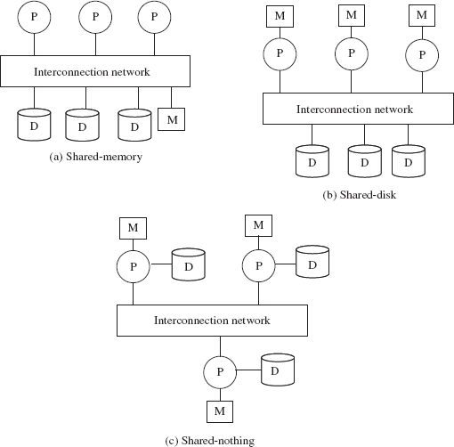
Fig. 13.1 Parallel database architecture

There are two important metrics for measuring the efficiency of a parallel database system, namely, scaleup and speedup. Running a task in less time by increasing the degree of parallelism is called speedup, and handling larger task by increasing the degree of parallelism is called scaleup.

13.2 DISTRIBUTED DBMS

In a distributed database system, data is physically stored across several computers. The computers are geographically dispersed and are connected with one another through various communication media (such as high-speed networks or telephone lines). Due to the distribution of data on multiple machines, potential exists for distributed computing which means the processing of a single task by several machines in a coordinated manner.

The computers in a distributed system are referred to as sites. In a distributed database system, each site is managed by a DBMS that is capable of running independent of other sites. The overall distributed system can be regarded as a kind of partnership among the individual local DBMSs at the individual local sites. The necessary partnership functionality is provided by a new software system at each site. This new software is logically an extension of local DBMS. The combination of this new software together with the existing DBMSs is called distributed DBMS (DDBMS). DDBMS permits the management of the distributed database and makes the distribution transparent to its users.

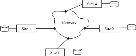
Fig. 13.2 A distributed database system

The shared-nothing parallel database system resembles distributed database system. The main difference is that former is implemented on tightly coupled multiprocessor and comprises a single database system. While in the latter, databases are geographically separated across the sites that share no physical components and are separately administered. The other difference is in their mode of operation. In shared-nothing architecture, there is symmetry and homogeneity of sites. However, in distributed database system, there may be heterogeneity of hardware and operating system at each site.

Homogeneous and Heterogeneous DDBMS

The distributed database system in which all sites share a common global schema and run the identical DBMS software and is known as homogeneous distributed database system. In such a system, DBMS software on different sites are aware of one another, and agree to work together in processing a user request at any site exactly as if data were stored at the user’s own site. In addition, the software must agree in exchanging information about transactions so that a transaction can be processed across multiple sites. Local sites relinquish a certain degree of control in terms of their right to change schemas or database-management system software to some other site.

On the other hand, a distributed database system in which different sites may have different schemas and run different DBMS software essentially autonomously is known as heterogeneous distributed database system or multidatabase system. In such a system, the sites may not be aware of one another and may provide limited facilities for cooperation in transaction processing. The differences in schemas also causes problem in query processing. In addition, differences in software obstruct the processing of transactions that access multiple sites.

13.2.1 Advantages of Distributed Database System

The distributed database system has various advantages ranging from decentralization to autonomy. Some of the advantages are as follows.

• Sharing data: The primary advantage of DDBMS is the ability to share and access data in an efficient manner. DDBMS provides an environment where users at a given site are able to access data stored at other sites. For example, consider an organization having many branches. Each branch stores data related to that branch; however, a manager of a particular branch can access information of any branch.
• Improved availability and reliability: Distributed systems provide greater availability and reliability. Availability is the probability that the system is running continuously throughout a specified period whereas reliability is the probability that the system is running (not down) at any given point of time. In distributed database systems, since, data is distributed across several sites, failure of a single site does not halt the entire system. The other sites can continue to operate in case of failure of one site. Only the data that exist at the failed site cannot be accessed. This means, some of the data may be inaccessible but other parts of database may still be accessible to the users. Furthermore, if the data is replicated at one or more sites, further improvement can be achieved.
• Autonomy: The possibility of local autonomy is the major advantage of distributed database system. Local autonomy implies that all operations at a given site are controlled by that site. It should not depend on any other site. Further, the security, integrity, and representation of local data are under the control of local site.
• Easier expansion: Distributed systems are more modular, hence, they can be expanded easily as compared to centralized systems, where upgrading a system with changes in hardware and software affects the entire database. In distributed system, the size of the database can be increased, and more processors or sites can be added as needed with little effort.

13.2.2 Distributed Database Storage

In distributed DBMS, the relations are stored across several sites. Accessing a relation that is stored at remote site increases the overhead due to exchange of messages. This overhead can be reduced by using two different techniques namely, fragmentation and replication. In fragmentation, a relation is divided into several fragments (or smaller relations), and each fragment can be stored at sites where they are more often accessed. In replication, several identical copies or replicas of each relation are maintained and each replica is stored at many distinct sites. Generally, replicas are stored at the sites where they are in high demand.

Note that a relation can be divided into several fragments and there may be several replicas of each fragment. In other words, both the techniques can be combined. These techniques are used during the process of distributed database design.

Fragmentation

Fragmentation of a relation R consists of breaking it into a number of fragments R1, R2, …, Rn such that it is always possible to reconstruct the original relation R from the fragments R1, R2, …, Rn. The fragmentation can be vertical or horizontal (see Figure 13.3).

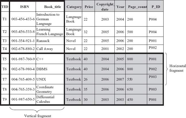
Fig. 13.3 Horizontal and vertical fragmentation

• Horizontal fragmentation: Horizontal fragmentation breaks a relation R by assigning each tuple of R to one or more fragments. In horizontal fragmentation, each fragment is a subset of the tuples in the original relation. Since each tuple of a relation R belongs to at least one of the fragments, original relation can be reconstructed. Generally, a horizontal fragment is defined as a selection on the relation R. That is, the tuples that belong to the horizontal fragment are specified by a condition on one or more attributes of the relation. For instance, fragment Ri can be constructed as shown here.

  Ri = σcondition(i) (R)

  The relation R can be reconstructed by applying union on all fragments, that is,

  R = R1 ∪ R2 ∪ … ∪ Rn

  For example, the relation book can be divided into several fragments on the basis of attribute Category as shown here.

  BOOK1 = σCategory = “Novel” (BOOK)
  BOOK2 = σCategory = “Textbook” (BOOK)
  BOOK3 = σCategory = “LanguageBook” (BOOK)

  Here, each fragment consists of tuples of BOOK relation that belongs to a particular category. Further, the fragments are disjoint. However, by changing the selection condition, a particular tuple of R can appear in more than one fragment.

• Vertical fragmentation: Vertical fragmentation breaks a relation by decomposing schema of relation R. In vertical fragmentation, each fragment is a subset of the attributes of the original relation. A vertical fragment is defined as a projection on the relation R as shown here.

  Ri = πRi (R)

  The relation should be fragmented in such a way that original relation can be reconstructed by applying natural join on the fragments. That is,

  R = R1 R2 … Rn

  To ensure the reconstruction of a relation from the fragments, one of the following options can be used.

  • include key attributes of R in each fragment Ri.
  • add a unique tuple id to each tuple in the original relation—this id is attached to each vertical fragment.
• Mixed fragmentation: Horizontal as well as vertical fragmentation can be applied to a single schema. That is, the fragments obtained by horizontally fragmenting a relation can be further partitioned vertically or vice-versa. This type of fragmentation is called mixed fragmentation. The original relation is obtained by the combination of join and union operations.

Replication

Replication means storing a copy (or replica) of a relation or relation fragments in two or more sites. Distribution of an entire relation at all sites is known as full replication. When only some fragments of a relation are replicated, it is called partial replication. In partial replication, the number of copies of each fragment can range from one to the total number of sites in the system.

Replication is desirable for the following two reasons.

• Increased availability of data: If a site containing the relation R fails, then the same relation can be found as long as at least one replica is available at some other site. Thus, the system can continue to process queries involving R, despite the failure of one site. Further, if the local copies of remote relations are available, we are less vulnerable to failure of remote site.
• Better performance: The system can process queries faster by operating on local copy of relation instead of communicating with remote sites. Moreover, if the majority of accesses to relation R require only reading of the relation, then several sites can process query involving R in parallel. In case there are more replicas of a relation, the probability of the needed data at the site where the transaction is initiated is more. Thus, data replication minimizes the overhead due to the movement of data between sites.

The major disadvantage of replication is that update operations incur greater overhead. The system must ensure that all the replicas of a relation are consistent to avoid erroneous results. Thus, whenever R is updated, all the replicas of R must be updated. For example, in an airline reservation system where the information regarding a flight is replicated at different sites, it is necessary that the information must agree in all sites.

In general, replication improves the performance of read operations in a distributed system and improves its reliability. However, the requirement that all the replicas must be updated makes the distributed database system more complex. In addition, concurrency control is more complicated.

Transparency

In a distributed system, the users should be able to access the database exactly as if the system were local. Users are not required to know where the data is physically stored and how the data can be accessed at the specific local site. Hiding all such details from the users is referred to as data transparency. DDBMS provides following type of transparencies.

• Location transparency (also known as location independence): Users should not know the physical location of the data. Users should be able to access the data as if all the data were stored at their own local site.
• Fragmentation transparency (also known as fragmentation independence): User should not be aware of the data fragmentation.
• Replication transparency (also known as replication independence): User should not be aware of the data replication. Data may be replicated either for better availability or performance. Users should be able to work as if data is not replicated at all.
• Naming transparency: Data items such as relations, fragments, and replicas must have unique names. This property can be ensured easily in a centralized system. However, in a distributed database, care must be taken to ensure that no two sites have same name for distinct data items. So that once a name is assigned to a data item, that named data item can be accessed unambiguously.

Data transparency is desirable because it simplifies application programs and end-user activities. At any time, in response to changing requirements, data can be changed, the number of copies can vary, and these copies can migrate from site to site. Further, data can be refragmented and fragments can be redistributed. Data transparency allows performing all these operations on data without manipulating programs or activities.

13.2.3 Distributed Query Processing

There are various issues that are involved in processing and optimizing a given query in a centralized database system as discussed in Chapter 08. In a distributed system, several other factors must also be taken into account. One of them is the communication cost. Since in a distributed system, a query may require data from more than one site, this transmission of data entails communication cost. Another factor is the gain in performance, if parts of a query are processed in parallel at different sites.

This section discusses the communication cost reduction techniques for one of the most common relational algebra operations, the join. Further, the gain in performance from having several sites process parts of query in parallel is elaborated.

Simple Join Processing

The join operation is one of the most expensive operations to perform. Thus, choosing a strategy for join is the major decision in the selection of a query-processing strategy. Consider the following relational algebra expression.

πISBN,Price,P_ID,Pname (BOOKBOOK.P_ID=PUBLISHER.P_IDPUBLISHER)

Suppose relations BOOK and PUBLISHER are stored at sites S1 and S2, respectively, and the result is to be produced at site S3. Further, suppose that there are 500 tuples in BOOK where each tuple is 100 bytes long and 100 tuples in PUBLISHER where each tuple is 150 bytes long. Thus, the size of BOOK relation is 500 * 100 = 50,000 bytes and the size of PUBLISHER relation is 100 * 150 = 15,000 bytes. The result of this query has 500 tuples where each tuple is 75 bytes long (assuming that the attributes ISBN, Price, P_ID, Pname are 15, 6, 4, and 50 bytes long). For simplicity, assume that these two relations are neither replicated nor fragmented. The different possible strategies that can be employed for processing this query are following.

1. Transfer replicas of both the relations to site S3 and process the query at this site to obtain the result. In this strategy, a total of 50,000 + 15000 = 65,000 bytes must be transferred.
2. Transfer replica of relation PUBLISHER to site S1 for processing the entire query locally at site S1 and then ship result to site S3. In this strategy, the bytes equivalent to the size of the query result and the size of relation PUBLISHER must be transferred. That is, 37,500 + 15,000 = 52,500 bytes must be transferred.
3. Transfer replica of relation BOOK to site S2 for processing the entire query locally at site S2 and then ship result to site S3. In this case, 50,000 + 37,500 = 87,500 bytes must be transferred.

If minimizing the amount of data transfer is the criteria for optimization, the strategy 2 must be chosen. However, in addition to amount of data transfer, the optimal choice also depends on the communication cost between a pair of sites and the relative speed of processing at each site. Thus, none of the above strategies is always the best.

Semijoin

Semijoin strategy is used to reduce the communication cost in performing a join operation. The idea behind semijoin strategy is to reduce the size of a relation that needs to be transmitted and hence the communication costs. In this strategy, instead of sending entire relation, joining attribute of one relation is sent to the site where other relation is present. This attribute is then joined with the relation and then the join attributes along with the required attributes are projected and transferred back to the original site. For example, consider once again the following relational algebra expression.

πISBN,Price,P_ID,Pname (BOOKBOOK.P_ID=PUBLISHER.P_ID PUBLISHER)

where, BOOK and PUBLISHER are stored at different sites S1 and S2, respectively. Further, suppose that system needs to produce the result at site S2. This relational algebra expression can be evaluated using the strategy as follows:

1. Project the join attribute (P_ID) of PUBLISHER at site S2 and transfer it to S1. A total of 100 * 4 = 400 bytes will be transferred.
2. Join this transferred attribute with the BOOK relation and transfer the required attributes from the resultant relation to site S2. A total of 500 * 25 (size of attribute ISBN + size of attribute Price + size of attribute P_ID), that is, 12,500 bytes are required to be transferred.
3. Evaluate the expression by joining the transferred attributes with PUBLISHER relation at site S2.

Here, 12,900 (12,500 + 400) bytes are required to be transferred. This strategy is more advantageous if small fraction of tuples of BOOK relation participates in join. It is clear that using this strategy, network cost can be reduced to a greater extent.

 

Parallelism

Consider the evaluation of a query that involves join of four relations as follows:

R S T U

Suppose the relations R, S, T, and U are stored at sites S1, S2, S3, and S4, respectively. Assume that the result is to be obtained at site S1. The query can be evaluated in parallel by using the strategy given here.

Relation R is transferred to site S2 where R S can be evaluated. At the same time, relation T is transferred to site S4 where T U can be evaluated. Site S2 can ship tuples of R S to S1 as they are generated, instead of waiting for the entire join to be computed. Similarly, site S4 can ship tuples of T U to S1. Once tuples of R S and T U reach at S1, the computation of R S T U can start. Hence, the computation of the final join result at S1 can be done in parallel with the computation of R S at S2 and T U at S4.

13.2.4 Distributed Transactions

In a distributed system, a transaction initiated at one site can access and update data at several other sites too. The transaction that accesses and updates data only at the site where it is initiated is known as local transaction. The transaction that accesses and updates data from several sites or the site other than the site at which the transaction is initiated is known as global transaction. A transaction that requires data from remote sites is broken into one or more subtransactions. These subtransactions are then distributed to the appropriate sites for execution. Note that such subtransactions are executed independently at the respective sites. The site at which the transaction is initiated is referred to as coordinator site and the sites where subtransactions are executed are called participating sites.

Like centralized system, each site has its own local transaction manager (TM) that manages the execution of those transactions (subtransactions) that access data stored in that site. The transactions may be either a local transaction or part of a global transaction. In addition, there is a transaction coordinator at each site that is responsible for coordinating the execution of all the transactions initiated at that site. The overall system architecture is shown in Figure 13.4 in which a transaction T_i initiated at coordinator site Si requires data from a remote site Sj. As a result, a subtransaction T_ij is distributed at the site Sj.

Fig. 13.4 System architecture

As discussed in Chapter 09, transaction must preserve ACID properties to ensure the integrity of the data. The ACID properties for local transactions can be assured by using certain concurrency control and recovery techniques as discussed in Chapter 10 and Chapter 11, respectively. However, for global transactions, ensuring these properties is a complicated task because of data distribution. Thus, both the concurrency control and recovery techniques need some modification to conform the distributed environment.

13.2.5 Concurrency Control in Distributed Databases

In DDBMS, concurrency control has to deal with replicated data items. Variations of the concurrency control techniques of centralized database system are used in distributed environment. Several such possible techniques based on the locking and timestamp are presented in this section.

 

Distributed Locking

The various locking techniques (discussed in Chapter 10) can be applied in distributed systems. However, they need to be modified in such a way that the lock manager can deal with the replicated data.

Single Lock Manager In single lock manager technique, the system maintains a single lock manager that resides in any single chosen site and all the requests to lock and unlock the data items are sent to that site. When a transaction needs to acquire lock on a specific data item, it sends request to the site where the lock manager resides. The lock manager checks whether the lock can be granted immediately. If the lock can be granted, the lock manager sends a message to the site from which the request for lock was initiated. Otherwise, the request is delayed until it can be granted. In case of a read lock request, data item at any one of the sites (at which replica of data item is present) is locked in the shared mode and then read. In case of a write lock request, all the replicas of the data item are locked in exclusive mode and then modified.

The advantage of this approach is that it is relatively easy to implement as it is merely a simple extension of the centralized approach. Since all requests to lock and unlock data items are made at one site, deadlock can be detected by applying directed graph (discussed in Chapter 10) directly. This technique has certain disadvantages too. Firstly, sending all locking requests to a single site can overload that site which can cause bottleneck. Secondly, the failure of the site containing lock manager disrupts the entire system as all the locking information is kept at t hat site.

Distributed Lock Manager In distributed lock manager technique, each site maintains a local lock manager which is responsible for handling the lock and unlock request for those data items that are stored in that site. When a transaction needs to acquire lock on a data item (assume that data item is not replicated) that resides at site say S, a message is sent to the lock manager at site S requesting appropriate lock. If the lock request is incompatible with the current state of locking of the requested data item, the request is delayed. Once it has ascertained that the lock can be granted, the lock manager sends a corresponding message to the site at which the request was initiated.

This approach is also simple to implement and to a great extent, it reduces the degree to which the coordinator is a bottleneck. However, in this technique detecting deadlock is more complex. Since lock requests are directed to a number of different sites, there may be inter-site deadlocks even when there is no deadlock within a single site. Thus, the deadlock-handling algorithm needs to be modified to detect global deadlocks (deadlock involving two or more sites). The modified deadlock-handling algorithm will be discussed later in this section.

Primary Copy This technique deals with the replicated data by designating one copy of each data item (say, Q) as a primary copy. The site at which the primary copy of Q resides is called primary site of Q. All requests to lock or unlock Q are handled by the lock manager at the primary site, regardless of the number of copies existing for Q. If the lock can be granted, the lock manager sends a message to the site from which the request for lock was initiated. Otherwise, the request is delayed until it can be granted.

Using this technique, concurrency control for replicated data can be handled the same way as for unreplicated data. Furthermore, load of processing lock requests is distributed among various sites by having primary copies of different data items stored at different sites. The failure of one site affects only those transactions that need to acquire locks on data items whose primary copies are stored at the failed site. The other transactions are not affected.

Majority Locking In majority locking technique, majority of the copies must be locked in case of both read and write lock request for a data item. Lock request is sent to more than one–half of the sites that contain a copy of the required data item. The local manager at each site determines whether the lock can be granted or not and acts similarly as discussed in earlier techniques. In this technique, a transaction cannot operate on a data item until the lock has been granted on a majority of the replica of the data item. Further, any number of transactions can simultaneously acquire a read lock on a majority of the replicas of a data item, since a read lock is shareable. However, only one transaction can acquire a write lock on a majority of these replicas. No transaction can majority lock a data item in the shared mode if it is already locked in exclusive mode.

This technique is considered as a truly distributed concurrency control method, since most of the sites are involved in decision in locking process. However, this technique is more complicated to implement than earlier discussed techniques. It is because it has higher message traffic among sites. Another problem with this scheme is that in addition to the problem of global deadlocks due to the use of a distributed lock manager, deadlock can occur even if only one data item is being locked. To illustrate this, consider a system with four sites S1, S2, S3, and S4 having data replicated at all sites. Suppose that transactions T₁ and T₂ need to lock a data item Q in exclusive mode. Further, suppose that transaction T₁ succeeds in locking Q at sites S1, and S4, while transactions T₂ succeeds in locking Q at sites S2 and S3. Now, to acquire the third lock, each of the transactions must wait. Hence, a deadlock has occurred. However, this type of deadlock can be easily prevented by making all sites to request locks on the replicas of the data item in the predetermined order.

Timestamping

We know that locking technique suffers from two disadvantages: deadlock and low level of concurrency. Timestamping technique therefore can be used as an alternative to locking. Though it is more complex to implement than locking, it prevents deadlock from occurring by avoiding in the first place. The main idea behind timestamping approach is that each transaction in the system is assigned a unique timestamp to determine its serialization order. Various timestamping methods for a centralized system can also be used in the distributed environment. However, extension in the centralized technique to distributed technique requires a method to be developed for generating unique global timestamps.

For generating unique timestamps in distributed systems, there are two primary methods, namely, centralized and distributed.

• Centralized scheme: In this scheme, a single site is responsible for generating the timestamps. The site can use either a logical counter or value of its own clock for this purpose.
• Distributed scheme: In this scheme, each site generates a unique local timestamp by using either a logical counter or local clock. This unique local timestamp is concatenated with the site identifier (which must also be unique) to get a unique global timestamp (see Figure 13.5). Note that the order of concatenation is important. The site identifier must be at the least significant position so that the global timestamps generated in one site is not always greater than those generated in another site. That is, the transactions are always ordered on the basis of the time of their occurrence not on the basis of the site from which they are initiated.

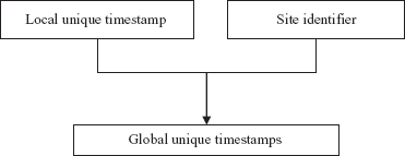
Fig. 13.5 Generation of global unique timestamps

Since the local timestamp is generated using local clock or logical counter, some problems can arise. If the logical counter is used, a relatively faster site would generate timestamps at a faster rate than the slower site. Thus, all the timestamps generated by the fast site will always be larger than those generated by another sites. Similarly, if the local clock is used, the timestamps generated by the site having fast clock will always be larger than those generated by another sites. So, some mechanism is required to keep these local timestamp generating schemes synchronized. It is accomplished by maintaining a logical clock at each site. Logical clock is implemented as a counter that is incremented after generating a new timestamp. This timestamp is included in the messages sent between sites. On receiving a message, the site compares its clock with this timestamp. If site finds that the current value of its logical clock is smaller than this message timestamp, it sets it to some value greater than the message timestamp.

Deadlock Handling

As stated earlier, in distributed systems, even when there is no deadlock within a single site, there may be inter-site deadlocks. In other words, deadlock involving two or more sites can occur. To illustrate this, consider a system having two sites S1 and S2 with following situation.

• At site S1, transaction T₁ is waiting to acquire lock on the data item held by transaction T₂. Transaction T₂ is waiting to acquire lock on the data item held by transaction T₄. Transaction T₃ is waiting to acquire lock on the data item locked by transaction T₁ and T₂.
• At site S2, transaction T₄ is waiting to acquire lock on the data item locked by transaction T₃.

The common deadlock-detection technique is wait-for graph. This technique requires that each site maintains its own local wait-for graph. The local wait-for graph [see Figure 13.6(a)] for both the sites S1 and S2 is constructed in the same way as discussed in Chapter 10. The only difference is that the nodes represent all the local as well as non-local transactions that are currently holding or requesting any of the items local to that site. Note that T₃ and T₄ are present in both the graphs indicating that transactions have requested data items at both sites.

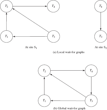
Fig. 13.6 Distributed deadlock

Observe that in Figure 13.6(a), each local wait-for graph is acyclic, indicating that there is no deadlock within the sites. However, absence of cycle in the local wait-for graph does not imply that there is no deadlock. This means, global deadlock cannot be detected solely on the basis of local wait-for graph.

To detect such deadlocks, the wait-for graph technique needs some extended treatment. In a distributed system, this technique requires generating not only local wait-for graph but also global wait-for graph for the entire system. Global wait-for graph [see Figure 13.6(b)] is constructed simply by the union of the local wait-for graphs and maintained at a single chosen site. Since this site is responsible for handling global deadlocks, it is known as deadlock detection coordinator.

The disadvantage of this technique is that it incurs communication overhead, as it requires sending all local wait-for graphs to the coordinator site. The other disadvantage is that delays in propagating local wait-for graphs may cause deadlock detection algorithms to identify deadlocks that do not really exist. Such deadlocks are known as phantom deadlocks. These types of deadlocks may lead to unnecessary rollbacks.

Instead of using one site for deadlock detection, it is possible to detect deadlock in a distributed manner. That is, several sites can take part in detecting deadlocks. In this technique, local wait-for graphs are sent to all the sites to generate only the concerned portion of global wait-for graph. However, such technique is more complicated to implement and sometimes deadlock may not be detected.

One other simple technique that can be used is time-out based technique. Recall that this technique falls between the deadlock prevention where a deadlock can never happen, and deadlock detection and recovery. In this technique, a transaction is allowed to wait for a fixed interval of time for required data item. If a transaction waits longer than specified time interval, it is aborted. Though this algorithm may cause unnecessary restarts, the overhead of deadlock detection is low. Moreover, if the participating sites do not cooperate to the extent of sharing their waits-for graphs, it may be the only option.

NOTE Deadlock prevention techniques can also be used for handling deadlocks but they may result in unnecessary delays and rollbacks. Thus, instead of deadlock prevention techniques, deadlock detection techniques are widely used.

13.2.6 Recovery in Distributed Databases

Recovery in a distributed system is more complicated than in a centralized system. In addition to the same type of failures encountered in a centralized system, a distributed system may suffer from new types of failures. The basic types of failures are loss of messages, failure of the site at which subtransaction is executing, and failure of communication links. The recovery system must ensure atomicity property, that is, either all the subtransactions of a given transaction must commit or abort at all sites. This property must be guaranteed despite any kind of failure. This guarantee is achieved using commit protocol. The most widely used commit protocol is the two-phase commit protocol (2PC).

Two-Phase Commit

In a distributed system, since a transaction is being executed at more than one site, the commit protocol may be divided into two phases, namely, voting phase and decision phase. To understand the operation of this protocol, consider a transaction T initiated at site Si where the transaction coordinator is Ci. When T completes its execution, that is, all the sites at which T has executed inform Ci that T has completed, Ci initiates the 2PC protocol. The two phases of this protocol are as follows:

• Voting phase: In this phase, the participating sites vote on whether they are ready to commit T or not. During this phase, the following actions are taken.
  1. Ci inserts a prepare record [T, prepare] in the log and force-writes the log onto stable storage. After this, Ci sends the prepare T message to all the participating sites.
  2. When the transaction manager at a participating site receives the prepare T message, it determines whether the site is ready to commit T or not. If the site is ready to commit T, it inserts a [T, ready] record in the log; otherwise it inserts [T, not-ready] record. It then force-writes the log onto stable storage and sends the ready T or abort T message to Ci accordingly.

  NOTE Any participating site can unilaterally decide to abort T before sending ready T message to the coordinator.

   

• Decision phase: In this phase, the coordinator site decides whether the transaction T can be committed or it has to be aborted. The decision is based on the responses to prepare T message that Ci receives from all the participating sites. The following responses may be received at the coordinator site.

1. A ready T message from all the participating sites. In this case, Ci decides to commit the transaction and inserts [T, commit] record to the log. It then force-writes the log onto stable storage and sends commit T message to all the participating sites.
2. At least one not-ready T message or no response from any participating site within the specified time-out interval. In this case, Ci decides to abort the transaction and inserts [T, abort] record to the log. It then force-writes the log onto stable storage and sends abort T message to all the participating sites.

Once the participating sites receive either the commit T or abort T message from Ci, they insert the corresponding record to the log, and force-write the log onto stable storage. After that, each participating site sends an acknowledge T message to Ci. Upon receiving this message from all the sites, Ci force-writes the [T, complete] record to the log.

NOTE As soon as the coordinator receives one abort T message, the coordinator decides to abort the transaction without waiting for other sites or time-out period.

 

Now, there may be a case that any site fails during the execution of the commit protocol. If any participating site fails, there are two possibilities. First, the site fails before sending ready T message. In this case, the coordinator does not receive any reply within the specified time interval. Thus, the transaction is aborted. Secondly, if the site fails after sending ready T message, the coordinator simply ignores the failure of participating site and proceeds in the normal way.

When the participating site restarts after failure, the recovery process is invoked. During recovery, the site examines its log to find all those transactions that were executing at the time of the failure. To decide the fate of those transactions, the recovery process proceeds as follows:

• If the log contains the [T, commit] or [T, abort] record, the site simply executes redo(T) or undo(T), respectively, and sends the acknowledgement T message to the coordinator.
• If the log contains the [T, ready] record, the site contacts the coordinator to determine whether to commit or abort T.
• If no such record exists in the log, the site decides unilaterally to abort the transaction and execute undo(T), since the site could not have voted before its failure.

Now, consider the case of coordinator’s failure. In this case, all the participating sites communicate with each other to determine the status of T. If any participating site contains the [T, commit] or [T, abort] record in its log, the transaction has to be committed or aborted, respectively. On the other hand, if any participating site does not contain [T, ready] record in its log, it means that site has not voted for T and without that vote, the coordinator could not have decided to commit T. Thus, in this case, it is preferable to abort T. However, if none of the discussed cases holds, the participating sites have to wait until the coordinator recovers, and all the locks acquired by T are held. This leads to blocking problem at the participating sites, since the transactions that require locks on data items locked by T have to wait.

When the coordinator restarts after failure, the recovery process is invoked at the coordinator site. The coordinator examines its log to determine the status of T.

• If the log contains [T, commit] or [T, abort] record, it executes redo(T) or undo(T), respectively, and periodically resends the commit T or abort T message to the participating sites, until it receives acknowledgement T message from each participating site.
• If the log contains [T, prepare] record, the coordinator unilaterally decides to abort T and conveys it to all the participating sites.

Three Phase Commit

The commit protocol called three-phase commit protocol (3PC), is an extension of the two-phase commit protocol that avoids blocking even if the coordinator site fails during recovery. To avoid blocking problem, this protocol requires some conditions which are as follows.

• There is no network partitioning.
• At least there is one available site.
• At most K sites fail, where K is some predetermined number.

If these conditions hold, 3PC protocol avoids blocking by introducing third phase between voting phase and the decision phase. In this phase, multiple sites are involved in the decision to commit. The basic idea of 3PC protocol is that when the coordinator sends prepare T message and receives yes votes from all the participant sites; it sends all participants pre-commit message instead of commit message. After ensuring that at least K other participating sites know about the decision to commit, the coordinator force-writes a commit log record and sends a commit message to all participants. The coordinator effectively postpones the decision to commit until it is sure that enough sites know about the decision to commit.

If the coordinator site fails, the other sites choose a new coordinator. This new coordinator communicates with the remaining other sites to check whether the old coordinator had decided to commit. It can be detected easily if any one of the other K sites that received pre-commit message is up. In this case, new coordinator restarts the third phase. If none of them has received pre-commit message, new coordinator aborts the transaction; otherwise, commits the transaction.

The 3PC protocol incurs an overhead during normal execution and requires that communication link failures do not lead to network partition to ensure freedom from blocking. For these reasons, it is not widely used.

 

13.3 CLIENT/SERVER SYSTEMS

As we know client/sever refers to the architecture where overall system is divided into two parts, client and server. They can run on two different machines. Thus, there is possibility of distributed computing. In fact, a client/server system can be considered as a special case of distributed system in which some sites are server sites and some are client sites; data resides at the server sites and all applications execute at the client sites.

In the late 1980s and early to mid of 1990s, a true distributed database system (that implement all the functionality discussed so far) was not a commercially feasible product. Thus, instead of making effort on developing a true distributed DBMS product, the vendors developed the distributed database system based on the client/server architecture. Two-tier client/server architecture can also be used for distributed system. However, it has some limitations. So, nowadays, three-tier client/server architecture has been used in developing distributed systems, particularly in web applications. The three-tier client/server architecture has already been introduced in Chapter 01. Here, all the three layers, namely, presentation layer, application layer, and database server of this architecture are explained in context of web applications. Different technologies related to each layer are given in Figure 13.7.

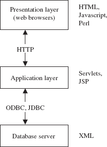
Fig. 13.7 Three-tier architecture for web applications with respective technologies

• Presentation layer (client): This layer provides an interface to handle user input and displays the needed information. At this layer, web interfaces or forms are provided through which the user can issue request, provide input, and the formatted output generated by application layer is displayed. For this purpose, Web browsers are used. HTML is the basic data presentation language that is used to communicate data from the presentation layer to the application layer. The other languages which can be used are Java, JavaScript, etc. This layer communicates with the application layer via HTTP protocol.
• Application layer: This layer executes the business logic of the application. It controls what data needs to input before an action can be executed, and what action are taken under what conditions. It issues SQL queries to the database server, formats the query result and sends to the client for presentation. The languages that can be used to program business logic are Java servlets, JSP, etc. This layer can communicate with one or more databases using standards such as ODBC, JDBC, etc. Apart from the business logic, it also handles functionality like security checks, identity verification, and so on.
• Database server: This layer processes the query requested by the application layer and send the results to it. Thus, it is the layer that accesses data from the database system. Generally, SQL is used to access the database if it is relational or object-relational. Stored procedures can also be used for the same purpose. At this level, XML may be used to exchange information regarding the query between the application server and the database server.

There are various approaches that are used to divide the DBMS functionality across client, application server, and database server. The common approach is to include the functionality of centralized database at the database server. The application server formulates SQL queries and connects to the database server when required. The client provides interfaces for user interactions. A number of relational products have adopted this approach.

1. The applications such as geographical information systems, computer-aided design, and real-time decision making demand the capability to manage data size of several hundred gigabytes to terabytes.
2. With the evolution of Internet, the number of online users as well as size of data has been increased. This demand has been the driving force of the emergence of technologies like parallel processing and data distribution.
3. The simultaneous use of computer resources such as CPUs and disks to perform a specific task is known as parallel processing. In parallel processing, many tasks are performed simultaneously on different CPUs.
4. The database systems based on parallelism and data distribution are called parallel DBMS and distributed DBMS.
5. Parallel DBMS seeks to improve performance by carrying out many operations in parallel, such as loading data, processing queries, and so on.
6. The three main architectures for building parallel database systems are shared–memory, shared–disk, and shared-nothing.
7. In distributed database system, data is physically stored across several computers. The computers are geographically dispersed and are connected with one another through various communication media (such as high-speed networks or telephone lines).
8. In distributed database system, each site is managed by a DBMS that is capable of running independent of other sites. The overall distributed system can be regarded as a kind of partnership among the individual local DBMSs at the individual local sites.
9. The necessary partnership functionality is provided by a new software system at each site. The combination of this new software together with the existing DBMSs is called distributed database management system (DDBMS).
10. The distributed database system, in which all sites run the identical DBMS software, is known as homogeneous distributed database system.
11. A distributed database system in which different sites may have different schemas and run different DBMS software, essentially autonomously, is known as heterogeneous distributed database system or multidatabase system.
12. In distributed DBMS, the relations are stored across several sites using two different techniques namely, fragmentation and replication.
13. In fragmentation, relation is divided into several fragments (or smaller relations), and each fragment can be stored at sites where they are more often accessed.
14. The fragmentation can be vertical or horizontal.
15. Horizontal fragmentation breaks a relation R by assigning each tuple of R to one or more fragments. Since each tuple of a relation R belongs to at least one of the fragments, original relation can be reconstructed. Generally, a horizontal fragment is defined as a selection on the relation R.
16. Vertical fragmentation breaks a relation by decomposing schema of relation R. In vertical fragmentation, each fragment is a subset of the attributes of the original relation.
17. The relation should be fragmented in such a way that original relation can be reconstructed by applying natural join on the fragments.
18. Horizontal as well as vertical fragmentation can be applied to a single schema. That is, the fragments obtained by horizontally fragmenting a relation can be further partitioned vertically or vice-versa. This type of fragmentation is called mixed fragmentation.
19. In replication, several identical copies or replicas of each relation are maintained and each replica is stored at many distinct sites. Generally, replicas are stored at the sites where they are in high demand.
20. Replication improves the performance of read operations in a distributed system and improves its reliability. However, updates incur greater overhead and the requirement that all the replicas be updated makes distributed database system more complex.
21. Users are not required to know where the data is physically stored and how the data can be accessed at the specific local site. Hiding all such details from the users is referred to as data transparency.
22. In a distributed system, several other factors must also be taken into account other than the communication cost. Since in a distributed system, a query may require data from more than one site, this transmission of data entails communication cost. Another factor is the gain in performance, if parts of a query are processed in parallel at different sites.
23. Various techniques are used in processing a query. The optimal choice depends on the communication cost between a pair of sites and the relative speed of processing at each site, in addition to the size of the data and the result being transferred.
24. The join operation is one of the most expensive operations to perform. Thus, choosing a strategy for join is the major decision in the selection of a query-processing strategy.
25. Semijoin strategy is used to reduce the communication cost in performing a join operation.
26. A transaction must preserve ACID properties to ensure the integrity of the data. The ACID properties for local transactions can be assured by using certain concurrency control and recovery techniques of centralized database system.
27. For global transactions, ensuring these properties is a complicated task because of data distribution. Thus, both the concurrency control and recovery techniques need some modification to conform the distributed environment.
28. In distributed systems, even when there is no deadlock within a single site, there may be inter-site deadlocks. To detect such deadlocks, the wait-for graph technique requires generating not only local wait-for graph but also global wait-for graph.
29. In addition to the handling new type of failures encountered in a centralized system, the recovery system must ensure atomicity property. This property must be guaranteed despite any kind of failure. This guarantee is achieved using commit protocol. The most widely used commit protocol is the two-phase commit protocol (2PC).
30. The commit protocol called three-phase commit protocol (3PC) is an extension of the two-phase commit protocol that avoids blocking even if the coordinator site fails during recovery.
31. A client–server system can be considered as a special case of distributed system in which some sites are server sites and some are client sites, data resides at the server sites, and all applications execute at the client sites.
32. Nowadays, three-tier client/server architecture has been used in developing distributed systems, particularly in web applications.

• Parallel processing
• Parallel database architecture
• Shared-memory architecture
• Shared-disk architecture
• Shared-nothing architecture
• Speedup
• Scaleup
• Distributed computing
• Distributed database management system (DDBMS)
• Homogeneous distributed database system
• Heterogeneous distributed database system or multidatabase system
• Fragmentation
• Horizontal fragmentation
• Vertical fragmentation
• Mixed fragmentation
• Replication
• Full replication
• Partial replication
• Data transparency
• Location transparency
• Fragmentation transparency
• Replication transparency
• Naming transparency
• Distributed query processing
• Semijoin
• Parallelism
• Distributed transactions
• Local transaction
• Global transaction
• Coordinator site
• Participating sites
• Distributed locking
• Single lock manager
• Distributed lock manager
• Primary copy
• Primary site
• Majority locking
• Timestamping
• Deadlock handling
• Local wait-for graph
• Global wait-for graph
• Deadlock detection coordinator
• Phantom deadlocks
• Commit protocol
• Two-phase commit protocol (2PC)
• Voting phase
• Decision phase
• Blocking problem
• Three-phase commit protocol (3PC)
• Three-tier client/server architecture
• Presentation layer
• Application layer
• Database sever

A. Multiple Choice Questions

1. Which of the following parallel database architectures resembles the distributed database system?
   1. Shared-memory
   2. Shared-disk
   3. Shared-nothing
   4. None of these
2. The important metric/s for measuring the efficiency of a parallel database system is
   1. Scaleup
   2. Speedup
   3. Both
   4. None of these
3. Which of the following transparencies means that users should be able to access the data as if all the data were stored at their own local site?
   1. Replication transparency
   2. Naming transparency
   3. Fragmentation transparency
   4. Location transparency
4. In which fragmentation, each fragment is a subset of the tuples in the original relation?
   1. Horizontal
   2. Vertical
   3. None of these
   4. Both
5. Which of the following is not an advantage of replication?
   1. Increased availability
   2. Reliability
   3. Better performance
   4. All of these
6. Which of the following conditions are required to avoid blocking problem by three-phase commit protocol (3PC) even if the coordinator site fails during recovery?
   1. There is no network partitioning.
   2. At least there is one available site.
   3. At most K sites fail, where K is some predetermined number.
   1. Both 1 and 2
   2. Both 2 and 3
   3. All of these
   4. None of these
7. Which of the following technologies is not related to presentation layer?
   1. JSP
   2. HTML
   3. Browsers
   4. Java
8. Which of the following techniques is considered as a truly distributed concurrency control method?
   1. Primary copy
   2. Majority locking
   3. Distributed lock manager
   4. Timestamping
9. Which of the following are the disadvantages of locking scheme?
   1. Low level of concurrency
   2. Deadlock
   3. Both (a) and (b)
   4. None of these
10. Which of these layers can communicate with one or more databases using standards such as ODBC, JDBC etc.?
    1. Presentation layer
    2. Application layer
    3. Database server
    4. None of these

B. Fill in the Blanks

1. The simultaneous use of computer resources such as CPUs and disks to perform a specific task is known as________________.
2. In ______________ architecture, each processor has a private memory and shares only storage disks via interconnection network.
3. ______________ strategy is used to reduce the communication cost in performing a join operation.
4. The site at which the transaction is initiated is referred to as ______________ and the sites where subtransactions are executed are called _______________.
5. Using _____________ technique, concurrency control for replicated data can be handled the same way as for unreplicated data.
6. The two phases of two phase commit protocol are___________ and _____________.
7. The delays in propagating local wait-for graphs may cause deadlock detection algorithms to identify deadlocks that do not really exist. Such deadlocks are known as ____________.
8. The recovery system must ensure ____________ property despite any kind of failure.
9. ______________ architecture has been used in developing distributed systems, particularly in web applications.
10. ____________ layer issues SQL queries to the database server, formats the query result and sends to the client for presentation.

C. Answer the Questions

1. Discuss the factors that motivate parallel and distributed database system.
2. Discuss the architecture of parallel database system.
3. What are distributed databases? How is data distribution performed in DDBMS?
4. What is the need of distributed database system? Give its two disadvantages.
5. Consider a bank that has a collection of sites, each running a database system. The databases interact by the electronic transfer of money between one another. Would such a system characterize as a distributed database? Why?
6. What is difference between shared-nothing parallel database system and distributed database system?
7. Explain the following terms:
   1. Distributed locking
   2. Fragmentation transparency
   3. Replication transparency
   4. Location transparency
8. When is it useful to have replication or fragmentation of data? Explain your answer.
9. Illustrate the issues to implement distributed database.
10. Discuss the different techniques for executing an equijoin of two relations located at different sites. What main factors affect the cost of data transfer?
11. Discuss the semijoin method for executing an equijoin of two relations at different sites. Under what conditions is an equijoin strategy efficient?
12. List all possible types of failure in a distributed system. Which of them are also applicable to a centralized system?
13. Suppose that a site gets no response from another site for a long time. Can the first site distinguish whether the connecting link has failed or the other site has failed? How is such a failure handled?
14. What is a commit protocol and why is it required in a distributed database? Describe and compare two phase and three phase commit protocol. What is blocking and how does the three phase protocol prevent it?
15. Explain how 2PC ensures transaction atomicity despite the failure for each possible failure.
16. Give an example of a distributed DBMS with three sites such that no two local waits-for graphs reveal a deadlock, yet there is a global deadlock.
17. Discuss deadlock detection techniques in a distributed database system.
18. What is a phantom deadlock? Give an example.
19. Consider a database of a company where a relation Employee (name, address, salary, branch) is fragmented horizontally by branch. Assume that each fragment has two replicas: one stored at site A and one stored locally at the branch site. Describe a good strategy for the following queries entered at site B.
    1. Find all employees at site C.
    2. Find the average salary of all employees.
    3. Find the lowest-paid employee in the company.
20. A bank has many branches. A customer can open his account in any branch and can operate his account from any branch. The information that is stored about account includes account number, branch, name of customer, address of customer, guarantors of the customer, balance.
    1. Suggest a suitable fragmentation scheme for the bank. Give reason in support of your scheme.
    2. Suggest a suitable replication scheme. Justify your suggestion. Make suitable assumptions, if any.
    3. Write at least two advantages and two disadvantages of data replication.