CHAPTER 8

QUERY PROCESSING AND OPTIMIZATION

A database management system manages a large volume of data which can be retrieved by specifying a number of queries expressed in a high-level query language such as SQL. Whenever a query is submitted to the database system, a number of activities are performed to process that query. Query processing includes translation of high-level queries into low-level expressions that can be used at the physical level of the file system, query optimization, and actual execution of the query to get the result. Query optimization is a process in which multiple query-execution plans for satisfying a query are examined and a most efficient query plan is identified for execution.

This chapter discusses the steps that are performed while processing a high-level query, the algorithms to implement various relational algebra operations and different techniques to optimize a query. It also discusses the operation called external sorting which is one of the primary and relatively expensive operations used in query processing.

8.1 QUERY PROCESSING STEPS

Query processing is a three-step process that consists of parsing and translation, optimization, and execution of the query submitted by the user. These steps are shown in Figure 8.1.

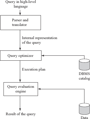
Fig. 8.1 Query processing steps

Whenever a user submits a query in high-level language (such as SQL) for execution, it is first translated into its internal representation suitable to the system. The internal representation of the query is based on the extended relational algebra. Thus, an SQL query is first translated into an equivalent extended relational algebra expression. During translation, the parser (portion of the query processor) checks the syntax of the user’s query according to the rules of the query language. It also verifies that all the attributes and relation names specified in the query are the valid names in the schema of the database being queried.

Just as there are a number of ways to express a query in SQL, there are a number of ways to translate a query into a number of relational algebra expressions. For example, consider a simple query to retrieve the title and price of all books with price greater than $30 from the Online Book database. This query can be written in SQL as given here.

  SELECT Book_title, Price
  FROM BOOK
  WHERE Price>30;

This SQL query can be translated into any of these two relational algebra expressions.

Expression 1: σPrice>30(ΠBook_title, Price(BOOK))

Expression 2: ΠBook_title, Price(σPrice>30(BOOK))

The relational algebra expressions are typically represented as query trees or parse trees. A query tree is a tree data structure in which the input relations are represented as the leaf nodes and the relational algebra operations as the internal nodes. When the query tree is executed, first the internal node operation is executed whenever its operands are available. Then the internal node is replaced by the relation resulted after the execution of the operation. The execution terminates when the root node is executed and the result of the query is produced. The query tree representations of the preceding relational algebra expressions are given in Figure 8.2(a).

Each operation in the query (such as select, project, join, etc.) can be evaluated using one of the several different algorithms, which are discussed in Section 8.3. The query tree representation does not specify how to evaluate each operation in the query. To fully specify how to evaluate a query, each operation in the query tree is annotated with the instructions which specify the algorithm or the index to be used to evaluate that operation. The resultant tree structure is known as query-evaluation plan or query-execution plan or simply plan. One possible query-evaluation plan for our example query is given in Figure 8.2(b). In this figure, the select operator σ is annotated with the instruction Linear Scan that specifies a complete scan of the relation.

Fig. 8.2 Query trees and query-evaluation plan

Different evaluation plans for a given query can have different costs. It is the responsibility of the query optimizer, a component of DBMS, to generate a least-costly plan. The metadata stored in the special tables called DBMS catalog is used to find the best way of evaluating a query. Query optimization is discussed in detail in Section 8.5. The best query-evaluation plan chosen by the query optimizer is finally submitted to the query-evaluation engine for actual execution of the query to get the desired result.

Query Blocks

Whenever a query is submitted to the database system, it is decomposed into query blocks. A query block forms a basic unit that can be translated into relational algebra expression and optimized. It consists of a single SELECT-FROM-WHERE expression. It also contains the GROUP BY and HAVING clauses if these are parts of the block. If the query contains the aggregate operators such as AVG, MAX, MIN, SUM, and COUNT, these operators are also included in the extended relational algebra.

In case of nested queries, each query within a query is identified as a separate query block. For example, consider an SQL query on BOOK relation.

  SELECT Book_title
  FROM BOOK
  WHERE Price > (SELECT MIN(Price)
                  FROM BOOK
                  WHERE Category=‘Textbook’);

This query contains a nested subquery and hence, is decomposed into two query blocks. Each query block is then translated into relational algebra expression and optimized. The optimization of nested queries is beyond the discussion of this chapter.

8.2 EXTERNAL SORT–MERGE ALGORITHM

Sorting of tuples plays an important role in database systems. It is discussed before other relational algebra operations because it is required in a variety of situations. Some of these situations are discussed here.

• Whenever an ORDER BY clause is specified in an SQL query, the output of the query needs to be sorted.
• Sorting is useful for eliminating duplicate values in the collection of records.
• Sorting can be applied on the input relations before applying join, union, or intersection operations on them to make these operations efficient.

If an appropriate index is available on a sort key, then there is no need to physically sort the relation as the index allows ordered access to the records. However, this type of ordering leads to a disk access (disk seek plus block transfer) for each record, which can be very expensive if the number of records is large. Thus, if the number of records is large, then it is desirable to order the records physically.

If a relation entirely fits in the main memory, in-memory sorting (called internal sorting) can be performed using any standard sorting techniques such as quick sort. If the relation does not fit entirely in the main memory, external sorting is required. An external sort requires the use of external memory such as disks or tapes during sorting. In external sorting, some part of the relation is read in the main memory, sorted, and written back to the disk. This process continues until the entire relation is sorted. Since, in general, the relations are large enough not to fit in the memory; this section discusses only the external sorting. The most commonly used external sorting algorithm is the external sort-merge algorithm (given in Figure 8.3). As the name suggests, the external sort-merge algorithm is divided into two phases, namely, sort phase, and merge phase.

• Sort phase: In this phase, the records in the file to be sorted are divided into several groups, called runs such that each run can fit in the available buffer space. An internal sort is applied to each run and the resulting sorted runs are written back to the disk as temporarily sorted runs. The number of initial runs (ni are computed as bR/M is the number of blocks containing records of relation R and M is the size of available buffer in blocks. If M = 5 blocks and bR = 20 blocks, then ni = 4 each of size 5 blocks. Thus, after the sorting phase 4 runs are stored on the disk as temporarily sorted runs.
• Merge phase: In this phase, the sorted runs created during the sort phase are merged into larger runs of sorted records. The merge continues until all records are in one large run. The output of merge phase is the sorted relation.

If ni>M, it is not possible to allocate a buffer for each sorted run in one pass. In this case, the merge operation is carried out in multiple passes. In each pass, M-1 buffer blocks are used as input buffers which are allocated to M-1 input runs and one buffer block is kept for holding the merge result. The number of runs that can be merged together in each pass is known as degree of merging (dM). Thus, the value of dM is the smaller of (M-1) or ni. If two runs are merged in each pass, it is known as two-way merging. In general, if N runs are merged in each pass, it is known as N-way merging.

      //Sort phase
           Load in M consecutive blocks of the relation.
              //M is number of blocks that can fit in main memory
           Sort the tuples in those M blocks using some internal sorting technique.
           Write the sorted run to disk.
           Continue with the next M blocks, until the end of the relation.
      //Merge phase (assuming that ni<M) //ni is the number of
                                        //initial runs
           Load the first block of each run into the buffer page of memory.
           Choose the first tuple (with the lowest value) among all the runs.
           Write the tuple to an output buffer page and remove it from the run.
           When the buffer page of any run is empty, load the next block of that run.
           When the output buffer page is full, write it to disk and start a new one.
           Continue until all buffer pages are empty.

Fig. 8.3 External sort-merge algorithm

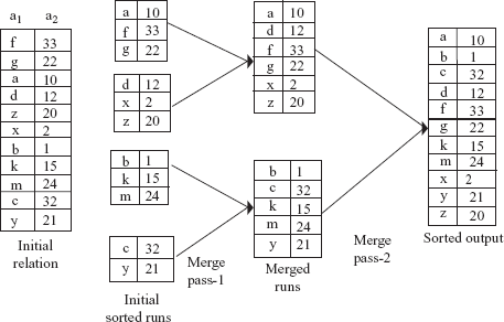
Fig. 8.4 An example of external sort-merge algorithm

An example of external sort-merge algorithm is given in Figure 8.4. We have assumed that the main memory holds at most three page frames out of which two are used as input and one for output during merge phase.

8.3 ALGORITHMS FOR RELATIONAL ALGEBRA OPERATIONS

The system provides a number of different algorithms for implementing several relational algebra operations. Several factors that influence which algorithm performs best include the sizes of the relations involved, existing indexes and sort orders, the size of available buffer pool, and the buffer replacement policy. These algorithms can be developed using any of these simple techniques.

• Indexing: In this technique, an index can be used to examine the tuples satisfying the condition specified in a select and join operation.
• Iteration: In this technique, all the tuples of a relation are examined one after the other. However, if the user wants only those attributes from the relation on which an index is defined, then instead of scanning all the tuples in the relation, the index data entries can be scanned.
• Partitioning: In this technique, the tuples are partitioned on the basis of a sort key. The two commonly used partitioning techniques are sorting and hashing.

Note that whichever technique is followed to develop an algorithm, the main aim is to minimize the cost of query evaluation. The cost of query evaluation depends on a number of factors such as seek time, number of block transfers between disk and memory, CPU time, storage cost, etc. For simplicity, we have given the cost functions in terms of number of block transfers only, and ignored all the other factors. In distributed or parallel database systems, the cost of communication is also included which is discussed in Chapter 13.

8.3.1 Implementation of Select Operations

The select operation is a simple retrieval of tuples from a relation. There are several algorithms for executing a select operation depending on the selection condition and the file being accessed. These algorithms are also known as file scans as they scan the records of the file to locate and retrieve the records satisfying the selection condition. In relational databases, if a relation is stored in a single, dedicated file, a file scan allows an entire relation to be read. If the search algorithm involves the use of indexes, it is known as index scan. This section discusses various algorithms for simple and complex select operations. The relational algebra expressions based on the Online Book database are given to illustrate the algorithms.

Implementing Simple Select Operations

If the selection condition does not involve any logical operator such as OR, AND, or NOT, it is termed as simple select operation. The algorithms to implement simple select operations are explained here.

• S1 (linear search): In linear search, every file block is scanned and all the records are tested to see whether their attribute values satisfy the selection condition. The linear search algorithm is also known as brute force algorithm. It is the simplest algorithm and can be applied to any file, regardless of the ordering of the file, or the availability of indexes. However, it may be slower than the other algorithms that are used for implementing selection. Since linear search algorithm searches all the blocks of the file, it requires bR block transfers, where bR is the total number of blocks of relation R.

  If the selection condition involves key attribute, the scan is terminated when the required record is found, without looking further at other records of the relation. The average cost in this case is equal to bR/2 block transfers if the record is found. In the worst case, the select operations involving key attribute may also require the scanning of all the records (bR block transfers) if no record satisfies the condition or the record is at the last location.

• S2 (binary search): If the file is ordered on an attribute and the selection condition involves an equality comparison on that attribute, binary search can be used to retrieve the desired tuples. Binary search is more efficient than the linear search as it requires scanning of lesser number of file blocks. For example, for the relational algebra operation σP_ID=“P002”(PUBLISHER), binary search algorithm can be applied if the PUBLISHER relation is ordered on the basis of the attribute P_ID.

  The cost of this algorithm is equal to log2(bR) block transfers. If the selection condition involves a non-key attribute, it is possible that more than one block contains the required records. Thus, the cost of reading the extra blocks has to be taken into account while estimating the cost.

Linear search and binary search are the basic algorithms for implementing select operation. If the tuples of a relation are stored together in one file, these algorithms can be used to implement the select operation. However, if indexes such as primary, clustering, or secondary indexes are available on the attributes involved in the selection condition, the index can be directly used to retrieve the desired record(s).

An index is also referred to as access path as it provides a path through which the data can be found and retrieved. Though indexes provide a fast, direct, and ordered access, they also add an extra overhead of accessing those blocks containing the index. The algorithms that use an index are described here.

• S3 (use of primary index, equality on key attribute): If the selection condition involves an equality comparison on a key attribute with a primary index, the index can be used to retrieve the record satisfying the equality condition. For example, for the relational algebra operation σP_ID=“P002”(PUBLISHER), the primary index on the key attribute P_ID (if available) can be used to directly retrieve the desired record. If B⁺-tree is used, the cost of this algorithm is equal to height of the tree plus one block transfer to retrieve the desired record.

   

  The select operation involving the equality comparison on the key attribute retrieves at most a single record, as a relation cannot contain two records with the same key value.

• S4 (use of clustering index, equality on non-key attribute): If the selection condition involves an equality comparison on the non-key attribute with a clustering index, the index can be used to retrieve all the records satisfying the selection condition. For example, for the relational algebra expression σP_ID=“P002”(BOOK), the clustering index on the non-key attribute P_ID of the BOOK relation (if available) can be used to retrieve the desired records. The cost of this algorithm is equal to the height of the tree plus the number of blocks containing the desired records, say b.
• S5 (use of secondary index, equality on key or non-key attribute): If the selection condition involves an equality condition on an attribute with a secondary index, the index can be used to retrieve the desired records. This search method can retrieve a single record if the indexing field is a key (candidate key) and multiple records if the indexing field is a non-key attribute. In the first case, only one record is retrieved, thus the cost is equal to height of the tree plus one block transfer to retrieve the desired record. In the second case, multiple records may be retrieved and each record may reside on a different disk blocks, thus, the cost is equal to the height of the tree plus n block transfers, where n is the number of records fetched.

  For example, for the relational algebra expression σPname=“Hills Publications”(PUBLISHER), secondary index on the candidate key Pname (if available) can be used to retrieve the desired record.

  The selection conditions discussed so far are equality conditions. The selection conditions involving comparisons can be implemented either by using a linear or binary search or by using indexes in one of these ways.

• S6 (use of primary index): If the selection condition involves comparisons of the form A>v, A>=v, A<v, or A<=v, where A is an attribute with a primary index and v is the attribute value, the primary ordered index can be used to retrieve the desired records. The cost of this algorithm is equal to the height of the tree plus bR/2 block transfers.
  • For comparison conditions of the form A>=v, the record satisfying the corresponding equality condition A=v is first searched using the primary index. A file scan starting from that record up to the end of file returns all the records satisfying the selection condition. For A>v, the file scan starts from the first tuple that satisfy the condition A>v—the record satisfying the condition A=v is not included.
  • For the conditions of the form A<v, the index is not searched, rather the file is simply scanned starting from the first record until the record satisfying the condition A=v is encountered. For A<=v, the file is scanned until the first record satisfying the condition A>v is encountered. In both the cases, the index is not useful.
• S7 (use of secondary index): The secondary ordered index can also be used for the retrievals based on comparison conditions such as <, <=, >, or >=. For the conditions of the form A<v or A<=v, the lowest-level index blocks are scanned from the smallest value up to v and for the conditions of the form A>v or A>=v, the index blocks are scanned from v up to the end of the file. The secondary index provides the pointers to the records and not the actual records. The actual records are fetched using the pointers. Thus, each record fetch may require a disk access, since records may be on different blocks. This implies that using the secondary index may even be more expensive than using the linear search if the number of fetched records is large.

Implementing Complex Select Operations

The selection conditions discussed so far are assumed to be simple conditions of the form A op B, where op can be =, <, <=, >, or >=. If the select operation involves complex conditions, made up of several simple conditions connected with logical operators AND (conjunction) or OR (disjunction), some additional algorithms are used.

• S8 (conjunctive selection using one index): If an attribute involved in one of the simple conditions specified in the conjunctive condition has an access path (such as indexes), any one of the selection algorithms S2 to S7 can be used to retrieve the records satisfying that condition. Each retrieved record is then checked to determine whether it satisfies the remaining simple conditions. The cost of this algorithm depends on the cost of the chosen algorithm.

  For example, for the relational algebra operation σP_ID=“P001” ∧ Category=“Textbook”(BOOK), if a clustering index is available on the attribute P_ID (algorithm S4), that index can be used to retrieve the records with P_ID=“P001”. These records can then be checked for the other condition. The records that do not satisfy the condition Category=“Textbook” are discarded.

• S9 (conjunctive selection using composite index): If a select operation specifies an equality condition on two or more attributes, the composite index (if available) on these combined attributes can be used to directly retrieve the desired records. For example, consider a relational algebra operation σR_ID=“A001” ∧ ISBN=“002-678-980-4”(REVIEW). If an index is available on the composite key (ISBN, R_ID) of the REVIEW relation, it can be used to directly retrieve the desired records.
• S10 (conjunctive selection by intersection of record pointers): If indexes or other access paths with record pointers (and not block pointers) are available on the attributes involved in the individual conditions, then each index can be used to retrieve the set of record pointers that satisfy an individual condition. The intersection of all the retrieved record pointers gives the pointers to the tuples that satisfy the conjunctive condition.

  For example, consider the relational algebra expression σP_ID=“P001” ∧ Category=“Textbook” BOOK). If secondary indexes are available on the attributes P_ID and Category of BOOK relation, then these indexes can be used to retrieve the pointers to the tuples satisfying the individual condition. The intersection of these record pointers yields the record pointers of the desired tuples. These records pointers are then used to retrieve the actual tuples (see Figure 8.5).

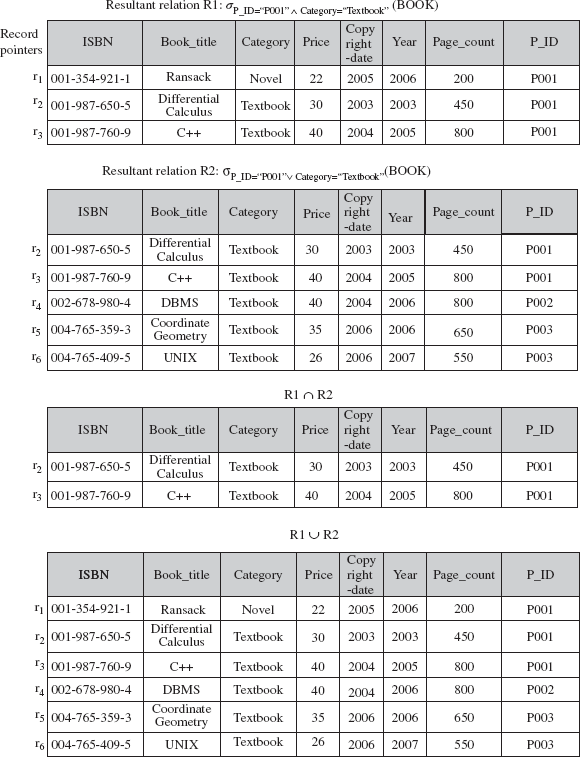
Fig. 8.5 An example of search algorithms S10 and S11

If indexes are not available for all the individual conditions, the retrieved records are further checked to determine whether they satisfy the remaining simple conditions. The cost of this algorithm is the cost of individual index scan plus the cost of retrieving the actual tuples. If the list of pointers is sorted before actually retrieving the actual tuples, this cost can be further reduced as it allows retrieval of the records in sorted order.

• S11 (disjunctive selection by union of record pointers): If indexes or other access paths are available on the attributes involved in the individual conditions, each index can be used to retrieve the set of record pointers that satisfy an individual condition. The union of all retrieved pointers gives the pointers to the tuples that satisfy the disjunctive condition.

  For example, consider the relational algebra expression σP_ID=“P001” v Category=“Textbook”(BOOK). If secondary indexes are available on the attributes P_ID and Category of BOOK relation, then these indexes can be used to retrieve the pointers to the tuples satisfying an individual condition. The union of these record pointers yields the pointers to the desired tuples. These records pointers are then used to retrieve the actual tuples (see Figure 8.5). If an index is not available on even one of the simple conditions, a linear search has to be performed on the relation to find the tuples that satisfy the disjunctive condition.

8.3.2 Implementation of Join Operations

The most time-consuming and complex operation in query processing is the join operation. If join operation is performed on two relations, it is termed as two-way join, and if more than two relations are involved in join, it is termed as multi way join. For simplicity, only two-way joins are discussed in this section. We will discuss various algorithms for join operation of the form RR.A=S.B S, where R and S are the two relations on which join operation is to be applied, and A and B are the domain-compatible attributes of R and S, respectively.

To understand the algorithms for join operations, consider the following operation on PUBLISHER relation of the Online Book database.

BOOKBOOK.P_ID = PUBLISHER.P_IDPUBLISHER

Further, assume the following information about these two relations. This information will be used to estimate the cost of each algorithm.

number of tuples of PUBLISHER=nPUBLISHER=2000

number of blocks of PUBLISHER=bPUBLISHER=100

number of tuples of BOOK=nBOOK=5000

number of blocks of BOOK=bBOOK=500

The various algorithms for implementing join operations are discussed here. For simplicity, the join condition BOOK.P_ID = PUBLISHER.P_ID is removed from all the expressions.

J1 (Nested-Loop Join)

The nested-loop join algorithm consists of a pair of nested for loops, one for each relation say, R and S. One of these relations, say R is chosen as the outer relation and the other relation S as the inner relation. The outer relation is scanned row by row and for each row in the outer relation the inner relation is scanned and looked for the matching rows. In other words, for each tuple r in R, every tuple s in S is retrieved and then checked whether the two tuples satisfy the join condition r[A]=s[B]. If the join condition is satisfied, then the values of these two tuples are concatenated, which is then added to the result. The tuple constructed by concatenating the values of the tuples r and s is denoted by r.s. Since this search scans the entire relation, it is also called naive nested loop join.

For natural join, this algorithm can be extended to eliminate the repeated attributes using a project operation. The nested-loop algorithms for equijoin and natural join operations are given in Figure 8.6. This algorithm is similar to the linear search algorithm for the select operation in a way that it does not require any indexes and it can be used with any join condition. Thus, it is also called brute force algorithm.

      for each tuple r in R do begin
           for each tuple s in S do begin
                      if r[A]=s[B] then add r.s to the result.
           end
      end

(a) Nested-loop join for equijoin operation

      for each tuple r in R do begin
           for each tuple s in S do begin
                if r[A]=s[B] then
                begin
                      delete one of the repeated attributes from the tuple r.s.
                      add r.s to the result.
                end
           end
      end

(b) Nested-loop join for natural join operation

Fig. 8.6 Nested-loop join

An extra buffer block is required to hold the tuples resulted from the join operation. When this block is filled, the tuples are appended to the disk file containing the join result (known as result file). This buffer block can then be reused to hold additional result records.

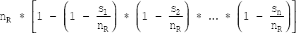
The nested-loop join algorithm is expensive, as it requires scanning of every tuple in S for each tuple in R. The pairs of tuples that need to be scanned are nR*nS, where nR and nS denote the number of tuples in R and S, respectively. For example, if PUBLISHER is taken as outer relation and BOOK as inner relation, 2000*5000 = 10⁷ pairs of tuples need to be scanned.

In terms of number of block transfers, the cost of this algorithm is equal to bR + (nR*bS), where bR and bS denote the number of blocks of R and S, respectively. For example, if PUBLISHER is taken as outer relation and BOOK is taken as inner relation, 100 + (2000 * 500)= 1,000,100 block transfers are required, which is very high. On the other hand, if BOOK is taken as outer relation and PUBLISHER as inner relation, then 500 + (5000 * 100) = 5,00,500 block transfers are required. Thus, by making the smaller relation as the inner relation, the overall costs of the join operation can be reduced.

If both or one of the relations fit entirely in the main memory, the cost of join operation will be bR+bS block transfers. This is the best-case scenario. For example, if either of the relations PUBLISHER and BOOK (or both) fits entirely in the memory, 100 + 500 = 600 block transfers are required, which is optimal.

J2 (Block Nested-Loop Join)

If the buffer is too small to hold either of the two relations entirely, the block accesses can still be reduced by processing the relations on a per-block basis rather than on a per-tuple basis. Thus, each block in the inner relation S is read only once for each block in the outer relation R (instead of once for each tuple in R). In the worst case, when neither of the relations fit entirely in the memory, this algorithm requires bR + (bR*bS) block transfers. It is efficient to use the smaller relation as the outer relation. For example, if PUBLISHER is taken as outer relation and BOOK as inner relation, 100 + (100 * 500) = 50,100 block transfers are required (which is much lesser than 1,000,100 or 5,00,500 block transfers as in the nested-loop join).

In the best case, where one of the relations fits entirely in the main memory, the algorithm requires bR+bS block transfers, which is same as that of nested-loop join. In this case, the smaller relation is chosen as the inner relation. The algorithm for block nested-loop join operation is given in Figure 8.7.

      for each block BR of R do begin
            for each block BS of S do begin
                 for each tuple r in BR do begin
                      for each tuple s in BS do begin
                           if r[A]=s[B] then
                                add r.s to the result.
                       end
                  end
            end
       end

Fig. 8.7 Block nested-loop join

J3 (Indexed Nested-Loop Join)

If an index is available on the join attribute of one relation say S, it is taken as the inner relation and the index scan (instead of file scan) is used to retrieve the matching tuples. In this algorithm, each tuple r in R is retrieved, and the index available on the join attribute of relation S is used to directly retrieve all the matching tuples. Indexed nested-loop join can be used with the existing as well as with a temporary index—an index created by the query optimizer and destroyed when the query is completed. If a temporary index is used to retrieve the matching records, the algorithm is called temporary indexed nested-loop join. If indexes are available on both the relations, the relation with fewer tuples can be used as the outer relation for better efficiency.

For example, if an index is available on the attribute P_ID of the BOOK relation, then the BOOK relation can be used as the inner relation. If a tuple with P_ID=“P001” exists in the PUBLISHER relation, then the matching tuples in the BOOK relation are those that satisfy the condition P_ID=“P001”. Since an index is available on P_ID, the matching tuples can be directly retrieved. The cost of this algorithm can be computed as bR+nR*c, where c is the cost of traversing the index and retrieving all the matching tuples of S. The algorithm for indexed nested-loop join operation is given in Figure 8.8.

      for each tuple r of R do begin
            probe the index on S to locate all tuples s such that
            s[B]=r[A].
            for each matching tuple s in S do
                            add r.s to the result.
      end

Fig. 8.8 Indexed nested-loop join

J4 (Sort-Merge Join)

If the tuples of both the relations are physically sorted by the value of their respective join attributes, the sort-merge join algorithm can be used to compute equijoins and natural joins. Both the relations are scanned concurrently in the order of the join attributes to match the tuples that have the same values for the join attributes. Since the relations are in sorted order, each tuple needs to be scanned only once and hence, each block is also read only once. Thus, if both the relations are in sorted order, the sort-merge join requires only a single pass through both the relations.

The number of block transfers is equal to the sum of number of blocks in both the relations R and S, that is, bR+bS. Thus, the join operation BOOKPUBLISHER requires 100 + 500 = 600 block transfers. If the relations are not sorted, they can be first sorted using external sorting. The sort-merge join algorithm is given in Figure 8.9(a) and an example of sort-merge join algorithm is given in Figure 8.9(b). In this figure, the relations R and S are sorted on the join attribute a1.

A variation of sort-merge algorithm can also be performed on unsorted relations if secondary indexes are available on the join attributes of both the relations. The records are scanned through indexes which allow the retrieval of records in sorted order. Since the records are physically scattered all over the file blocks, accessing each tuple may require accessing a disk block, which is very expensive.

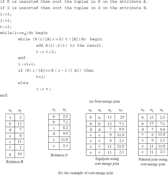
Fig. 8.9 Implementing sort-merge join

This cost can be reduced by using a hybrid merge-join technique which combines sort-merge join with indexes. To understand the hybrid merge-join algorithm, consider a sorted relation R and an unsorted relation S having a secondary B⁺-tree index on the join attribute. The tuples of sorted relation are merged with the leaf entries of the secondary B⁺-tree index. The result file in this case contains the tuples from the sorted relation and the addresses of the tuples of the unsorted relation. This result file is then sorted on the basis of the addresses of tuples of the unsorted relation. The corresponding tuples can then be retrieved in physical storage order to complete the join. If both the relations are unsorted, the addresses of the tuples of both the relations are merged and sorted, and the corresponding tuples are retrieved from both the relations in physical storage order.

J5 (Hash Join)

In this algorithm, a hash function h is used to partition the tuples of each relation into sets of tuples with each set containing tuples that have the same hash value on the join attributes A of relation R and B of relation S. The algorithm is divided into two phases, namely, partitioning phase and probing phase. In partitioning (also called building) phase, the tuples of relations R and S are partitioned into the hash file buckets using the same hash function h. Let Pr0, Pr1, …, Prn be the partitions of tuples in relation R and Ps0, Ps1, …, Psn be the partitions of tuples in relation S. Here, n is the number of partitions of relations R and S. The main property of hash join is that the tuples in the partition Pri need to be joined with tuples in the partition Psi. This is because of the fact that if tuples of relation R with some hash value hash to i, then the tuples of relation S with same hash value also hash to i.

During partitioning phase, a single in-memory buffer with size one disk block is allocated for each partition to store the tuples that hash to this partition. Whenever the in-memory buffer gets filled, its contents are appended to a disk sub file that stores this partition. For a simple two-way join, the partitioning phase has two iterations. In the first iteration, the relation R is partitioned into n partitions, and in second iteration, the relation S is partitioned in n partitions. In probing (also called matching or joining) phase, n iterations are required. In ith iteration, the tuples in the partition Pri are joined with the tuples in the corresponding partition Psi.

The hash join algorithm requires 3(bR+bS)+4n block transfers. The first term 3(bR+bS) represents that the block transfer occurs three times—once when the relations are read into the main memory for partitioning, second when they are written back to the disk and third, when each partition is read again during the joining phase. The second term 4n represents an extra overhead (2n for each relation) of reading and writing of each partition to and from the disk—since the number of blocks occupied by each partition is slightly more than bR+bS because of partially filled blocks. The extra overhead of 4n is generally very small as compared to bR+bS and hence, can be ignored.

The main difficulty of the algorithm is to ensure that the partitioning hash function is uniform, that is, it creates partitions of almost same size. If the partitioning hash function is non-uniform, then some partitions may have more tuples than the average, and they might not fit in the available main memory. This type of partitioning is known as skewed partitioning. This problem can be handled by further partitioning the partition into smaller partitions using a different hash function.

Recursive Partitioning and Hybrid Hash Join If the value of n is less than the value M-1 (M is the number of page frames in the main memory), the hash join algorithm is very simple and efficient to execute as both the relations can be partitioned in one pass. However, if the value n is greater than or equal to M, then the relations cannot be partitioned in a single pass, rather partitions have to be done in repeated passes.

In the first pass, the input relation is partitioned into M-1 partitions (one page frame is kept to be used as input buffer) using a hash function h. In the next pass, each partition created in the previous pass is partitioned again to create smaller partitions using a different hash function. This process is repeated until each partition of the input relation can fit entirely in the memory. This technique is called recursive partitioning. Note that a different hashing function is used in each pass. A relation S does not require recursive partitioning if M>√bS or equivalently M>n+1.

If memory size is relatively large, a variation of hash join called hybrid hash join can be used for better performance. In hybrid hash join technique, the probing phase for one of the partitions is combined with the partitioning phase. The main objective of this technique is to join as many tuples during the partitioning phase as possible in order to save the cost of storing these tuples back to the disk and accessing them again during the joining (probing) phase.

To better understand the hybrid hash join algorithm, consider a hash function h(K)=K mod n that creates n partitions of the relation, where n< M and consider the join operation BOOKPUBLISHER.

In the first iteration, the algorithm divides the buffer space among n partitions such that all the blocks of first partition of the smaller relation PUBLISHER completely reside in the main memory. A single input buffer (with size one disk block) is kept for each of the other partitions, and they are written back to the disk as in the regular hash join. Thus, at the end of the first iteration of the partitioning phase, the first partition of the relation PUBLISHER resides completely in the main memory and other partitions reside in a disk sub file.

In the second iteration of the partitioning phase, the tuples of the second relation BOOK are being partitioned. If a tuple hashes to the first partition, it is immediately joined with the matching tuple of PUBLISHER relation. If the tuple does not hash to the first partition, it is partitioned normally. Thus, at the end of the second iteration, all the tuples of BOOK relation that hash to the first partition have been joined with the tuples of PUBLISHER relation. Now, there are n-1 pairs of partitions on the disk. Therefore, during the joining phase, n-1 iterations are needed instead of n.

8.3.3 Implementation of Project Operations

A project operation of the form Π<attribute_list>(R) is easy to implement if the <attribute_list> includes the key attribute of the relation R. This is because in this case duplicate elimination is not required, and the result will contain the same number of tuples as R but with only the values of attributes listed in the <attribute_list>. However, if the <attribute_list> does not contain the key attribute, duplicate tuples may exist and must be eliminated. Duplicate tuples can be eliminated by using either sorting or hashing.

• Sorting: The result of the operation is first sorted, and then the duplicate tuples that appear adjacent to each other are removed. If external sort-merge technique is used, the duplicate tuples can be found while creating runs, and they can be removed before writing the runs on the disk. The remaining duplicate tuples can be removed during merging. Thus, the final sorted run contains no duplicates.
• Hashing: As soon as a tuple is hashed and inserted into in-memory hash file bucket, it is first checked against those tuples that are already present in the bucket. The tuple is inserted in the bucket if it is not already present, otherwise it is discarded. All the tuples are processed in the same way.

Note that the cost of duplicate elimination is very high. Thus, in SQL the user has to give an explicit request to remove duplicates using the DISTINCT keyword. The algorithm to implement project operation by eliminating duplicates using sorting is given in Figure 8.10.

      for each tuple r in R do
            add a tuple r[<attribute_list>] in T’.
                 //T’ may contain duplicate tuples
      if <attribute_list> includes the key attribute of R then
            T:=T’;     // T contains the projection result
                       // without duplicates
      else
      begin
            sort the tuples in T’.
            i:=1;
            j:=2;
            while(i<=nR) do begin
                  if (T’(i)[A]==T’(j)[A]) then
                        j:=j+1;
                  else begin
                        output the tuple T’[i] to T.
                        i:=j;
                  end
            end
      end

Fig. 8.10 Algorithm for project operation

8.3.4 Implementation of Set Operations

There are four set operations, namely, union, intersection, set difference, and Cartesian product. Generally, the Cartesian product operation R×S is quite expensive as it results in a large resultant relation with nR*nS tuples and j+k attributes (j and k are the number of attributes in R and S, respectively). Thus, it is better to avoid Cartesian product operation.

The other three set of operations, namely, union, intersection, and set difference can be implemented by first sorting the relations on the basis of same attribute and then scanning each sorted relation once to produce the result. For example, the operation R ∪ S can be implemented by concurrently scanning and merging both the sorted relations—whenever same tuple exists in both the relations, only one of them is kept in the merged result. The operation R ∩ S can be implemented by adding only those tuples to the merged result that exist in both the relations. Finally, the operation R – S is implemented by retaining only those tuples that exist in R but are not present in S.

If the relations are initially sorted in the same order, all these operations require bR+bS block transfers. If the relations are not sorted initially, the cost of sorting the relations has to be included. The algorithms for the operations R ∪ S, R ∩ S, and R – S using sorting are given in Figure 8.11.

Each of these operations can also be implemented using hashing as shown below.

Implementing R ∪ S

1. Partition the tuples of relation R into hash file buckets.
2. Probe (hash) each tuple of relation S, and insert the tuple in the bucket if no identical tuple from R is found in the bucket.
3. Add the tuples in the hash file bucket to the result.

Implementing R ∩ S

1. Partition the tuples of relation R into hash file buckets.
2. Probe (hash) each tuple of relation S, and if an identical tuple from R is already present in the bucket, then add that tuple to the result file.

Implementing R – S

1. Partition the tuples of relation R into hash file buckets.
2. Probe (hash) each tuple of relation S, and if an identical tuple from R is already present in the bucket, then remove that tuple from the bucket.
3. Add the tuples remaining in the bucket to the result file.

8.3.5 Implementation of Aggregate Operations

If the aggregate operators MIN, MAX, SUM, AVG, and COUNT are applied to an entire relation (that is, without using a GROUP BY clause), they can be computed either by scanning the entire relation or by using an index, if available. For example, consider the following operation.

Max(Price), MIN(Price)(BOOK)

If an index on the Price attribute of the BOOK relation exists, it can be used to search for the largest and the smallest price value. In case, the GROUP BY clause is included in the query, the aggregate operation can be implemented either by using sorting or hashing as done for duplicate elimination. The only difference is that instead of removing the tuples with the same value for the grouping attribute, these tuples are grouped together and the aggregate operations are applied on each group to get the desired result. The cost of implementing the aggregate operation is same as that of duplicate elimination.

      sort the tuples of R and S on the basis of same unique sort attributes.
      i:=1;
      j:=1;
      while(i<=nR) and (j<=nS) do begin
           if(R(i) < S(j)) then begin
                add R(i) to the result.
                i:=i+1;
           end
           elseif (R(i) > S(j)) then begin
                add S(j) to the result.
                j:=j+1;
           end
           else begin
                add R(i) to the result.
                i:=i+1;
                j:=j+1;    //R(i)=S(j), add only one tuple
           end
      end
      while(i<=nR) do begin
           add R(i) to the result.   //add remaining tuples
                                            //of R, if any
           i:=i+1;
      end
      while(j<=nS) do begin
           add S(j) to the result.   //add remaining tuples
                                            //of S, if any
           j:=j+1;
      end

(a) Implementing UNION operation

      sort the tuples of R and S on the basis of same unique sort attributes.
      i:=1;
      j:=1;
      while(i<=nR) and (j<=nS) do begin
           if(R(i) < S(j)) then
                i:=i+1;
           elseif(R(i) > S(j)) then
                j:=j+1;
           else begin
                //R(i)=S(j),add one of the tuples to the result
                add R(i) to the result.
                i:=i+1;
                j:=j+1;
           end
      end

(b) Implementing INTERSECTION operation

      sort the tuples of R and S on the basis of same unique sort attributes.
      i:=1;
      j:=1;
      while(i<=nR) and (j<=nS)do begin
           if(R(i) < S(j)) then begin
                add R(i) to the result.
                //R(i)has no matching S(j)
                //so add R(i) to the result
                i:=i+1;
           end
           if(R(i) > S(j)) then
                j:=j+1;
           else begin
                //R(i)=S(j) so skip both the tuples
                i:=i+1;
                j:=j+1;
           end
      end
      while(i<=nR) do begin
           add R(i) to the result.
                //add remaining tuples of R, if any
           i:=i+1;
      end

(c) Implementing SET DIFFERENCE operation

Fig. 8.11 Implementing set operations

The aggregate operations can also be implemented during the creation of the groups. For example, as soon as two tuples in the same group are found, these two tuples can be replaced with a single tuple containing the result of SUM, MIN, or MAX in the columns being aggregated. In case of COUNT operation, the system maintains a counter for each group and as soon as a tuple belonging to a particular group is found, the counter for that group is incremented by one. The AVG operation is implemented by dividing the sum and count values calculated using the method described earlier.

8.4 EXPRESSIONS CONTAINING MULTIPLE OPERATIONS

So far we have discussed how individual relational algebra operations are evaluated. This section discusses how the expressions containing multiple operations are evaluated. Such expressions are evaluated either using materialization approach or pipelining approach.

8.4.1 Materialized Evaluation

In materialized evaluation, each operation in the expression is evaluated one by one in an appropriate order and the result of each operation is materialized (created) in a temporary relation which becomes input for the subsequent operations. For example, consider this relation algebra expression.

ΠPname,Email_id(σCategory=“Novel”(BOOK)PUBLISHER)

This expression consists of three relational operations, join, select, and project. The query tree (also known as operator tree or expression tree) of this expression is given in Figure 8.12.

In materialization approach, the lowest-level operations (operations at the bottom of operator tree) are evaluated first. The inputs to the lowest-level operations are the relations in the database. For example, in Figure 8.12, the operation σCategory=“Novel”(BOOK) is evaluated first and the result is stored in a temporary relation. The temporary relation and the relation PUBLISHER are then given as inputs to the next-level operation, that is, the join operation. The join operation then performs a join on these two relations and stores the result in another temporary relation which is given as input to the project operation which is at the root of the tree.

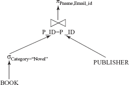
Fig. 8.12 Operator tree for the expression

A single buffer is used to hold the intermediate result and when it gets filled it is written back to the disk. If double buffering is used, the expression evaluation becomes fast. In double buffering, two buffers are used—one of them continues with the execution of the algorithm while the other being written to the disk. This allows CPU activity to perform in parallel with I/O activity. The cost of materialized evaluation is the sum of the costs of the individual operations involved plus the cost of writing the intermediate results to the disk.

8.4.2 Pipelined Evaluation

The main limitation of materialized evaluation is that it results in a number of temporary relations which affects the query-evaluation efficiency. To improve the efficiency of query evaluation, we need to reduce the number of temporary relations that are produced during query execution. This can be achieved by combining several operations into a pipeline or a stream of operations. This type of evaluation of expressions is called pipelined evaluation or stream-based processing. With pipelined evaluation, operations form a queue and results are passed from one operation to another as they are calculated. This technique thus avoids write-outs of the temporary relations.

For example, the operations given in Figure 8.12 can be placed in a pipeline. As soon as a tuple is generated from the select operation, it is immediately passed to the join operation for processing. Similarly, a tuple generated from the join operation is passed immediately to the project operation for processing. Thus, the evaluation of these three operations in a pipelined manner directly generates the final result without creating temporary relations. The system maintains one buffer for each pair of adjacent operations to hold the tuples being passed from one operation to the next. Since the results of the operations are not stored for a long time, lesser amount of memory is required in pipelining approach. However, the inputs are not available to the operations for processing all at once in the pipelining.

There are two ways of executing pipelines, namely, demand-driven pipeline and producer-driven pipeline.

• Demand-driven pipeline: In this approach, the parent operation requests next tuple from its child operations as required, in order to output its next tuple. Whenever an operation receives a request for the next set of tuples, it computes those tuples and then returns them. Since, the tuples are generated lazily, on demand; this technique is also known as lazy evaluation.
• Producer-driven pipeline: In this approach, each operation at the bottom of the pipeline produces tuples without waiting for the request from the next higher-level operations. Each operation then puts the output tuples in the output buffer associated with it. This output buffer is used as input buffer by the operation at next higher level. The operation at any other level consumes the tuples from its input buffer to produce the output tuples, and puts them in its output buffer. In any case, if the output buffer is full, the operation has to wait until tuples are consumed by the operation at the next higher-level. As soon as the buffer has some space for more tuples, the operation again starts producing the tuples. This process continues until all the tuples are generated. Since, the tuples are generated eagerly; this technique is also known as eager pipelining.

8.5 QUERY OPTIMIZATION

The success of relational database technology is largely due to the systems’ ability to automatically find evaluation plans for declaratively specified queries. The query submitted by the user can be processed in a number of ways especially if the query is complex. Thus, it is the responsibility of the query optimizer to construct a most efficient query-evaluation plan having the minimum cost.

To find the least-costly plan, the query optimizer generates alternative plans that produce the same result as that of the given expression and then chooses the one with the minimum cost. There are two main techniques of implementing query optimization, namely, cost-based optimization and heuristics-based optimization. Practical query optimizers incorporate elements of both these approaches. In addition to these approaches, another approach called semantic query optimization has also been introduced which is knowledge-based optimization. It makes use of problem-specific knowledge, represented as integrity constraints, to answer the queries efficiently.

8.5.1 Cost-Based Query Optimization

A cost-based query optimizer generates a number of query-evaluation plans from a given query using a number of equivalence rules, and then chooses the one with the minimum cost. The cost of executing a query include:

• cost of accessing secondary storage—cost of searching, reading, and writing disk blocks.
• storage cost—cost of storing intermediate results.
• computation cost—cost of performing in-memory operations.
• memory usage cost—cost related to the number of occupied memory buffers.
• communication cost—cost of communicating the query result from one site to another.

The cost of each evaluation plan can be estimated by collecting the statistical information about the relations such as relation sizes and available primary and secondary indexes from the DBMS catalog. This section discusses the various equivalence rules which are used to generate a set of expressions that are logically equivalent to the given expression, and the various techniques to estimate the statistics.

Equivalence Rules

An expression is said to be equivalent to a given relational algebra expression if, on every legal database instance, it generates the same set of tuples as that of original expression irrespective of the ordering of the tuples. For example, consider a relational algebra expression for the query “Retrieve the publisher name and category of the book C++”.

ΠPname,Category(σBook_title=“C++”(BOOK PUBLISHER))

The initial operator tree of this expression is given in Figure 8.13(a). It is clear from the initial operator tree of this expression that first the join operation is applied on the relations BOOK and PUBLISHER, which results in a large intermediate relation. However, the user is only interested in those tuples having Book_title=“C++”. Thus, another way to execute this query is to first select only those tuples from the BOOK relation satisfying the condition Book_title=“C++”, and then join it with the PUBLISHER relation. This reduces the size of the intermediate relation. The query can now be represented by the following expression.

ΠPname,Category(σBook_title=“C++”(BOOK) PUBLISHER)

Fig. 8.13 Initial and transformed operator trees

This expression is equivalent to the original expression; however, with less number of tuples in the intermediate relation and thus, it is more efficient. The transformed operator tree of the equivalent expression is given in Figure 8.13(b). Therefore, the main aim of generating logically equivalent expressions is to minimize the size of intermediate results.

Equivalence rules specify how to transform an expression into a logically equivalent one. An equivalence rule states that expressions of two forms are equivalent if an expression of one form can be replaced by expression of the other form, and vice versa. While discussing the equivalence rules it is assumed that c, c1, c2, …, cn are the predicates, A, A1, A2, …, An are the set of attributes and R, R1, R2, …, Rn are the relation names.

Rule 1: The selection condition involving conjunction of two or more predicates can be deconstructed into a sequence of individual select operations. That is,

  σc1 ∧ c2(R) = σc1(σc2(R))

This transformation is called cascading of select operator.

Rule 2: Select operations are commutative. That is,

  σc1(σc2(R)) = σc2(σc1(R))

Rule 3: If a query contains a sequence of project operations, only the final operation is needed, the others can be omitted. That is,

  ΠA1(ΠA2(…(ΠAn(R))…))= ΠA1(R)

This transformation is called cascading of project operator.

Rule 4: If the selection condition c involves only the attributes A1, A2, …, An that are present in the projection list, the two operations can be commuted. That is,

  ΠA1,A2,…,An(σc(R))= σc(ΠA1,A2,…,An(R))

Rule 5: Selections can be combined with Cartesian products and joins. That is,

1. σc(R1 X R2) = R1c R2
2. σc1(R1c2 R2) = R1c1 ∧ c2R2

Rule 6: Cartesian product and join operations are commutative. That is,

1. R1 X R2 = R2 X R1
2. R1c R2 = R2c R1

Note that the ordering of the attributes in the results of left-hand side and right-hand side expressions will be different. Thus, if the ordering is to be taken into account, the equivalence does not hold. In order to appropriately reorder the attributes, a project operator can be added to either of the side of equivalence. For simplicity, project operator is omitted and the attribute order is ignored in most of our examples.

Rule 7: Cartesian product and join operations are associative. That is,

1. (R1 X R2) X R3 = R1 X (R2 X R3)
2. (R1 R2) R3 = R1 (R2 R3)

Rule 8: The select operation distributes over the join operation in these two conditions.

1. If all the attributes in the selection condition c1 involve only the attributes of one of the relations (say, R1), then the select operation distributes. That is,

   σc1(R1 c R2)=(σc1(R1)) c R2

2. If the selection condition c1 involves only the attributes of R1 and c2 involves the attributes of R2, then the select operation distributes. That is,

   σc1 ∧ c2(R1 c R2) = (σc1(R1)) c(σc2(R2))

Rule 9: The project operation distributes over the join operation in these two conditions.

1. If the join condition c involves only the attributes in A1 ∪ A2, where A1 and A2 are the attributes of R1 and R2, respectively, the project operation distributes. That is,

   ΠA1 ∪ A2(R1 c R2) = (ΠA1(R1)) c (ΠA2(R2))

2. If the attributes A3 and A4 of R1 and R2, respectively, are involved in the join condition c, but not in A1 ∪ A2, then,

   ΠA1 ∪ A2(R1 c R2) = ΠA1 ∪ A2((ΠA1 ∪ A3(R1)) c(ΠA2 ∪ A4(R2)))

Rule 10: The set operations union and intersection are commutative and associative. That is,

1. Commutative

   R1 ∪ R2 = R2 ∪ R1
   R1 ∩ R2 = R2 ∩ R1

2. Associative

   (R1 ∪ R2) ∪ R3 = R1 ∪ (R2 ∪ R3)
   (R1 ∩ R2) ∩ R3 = R1 ∩ (R2 ∩ R3)

 

Rule 11: The select operation distributes over the union, intersection, and set difference operations. That is,

  σc(R1 ∪ R2) = σc(R1) ∪ σc(R2)
  σc(R1 ∩ R2) = σc(R1) ∩ σc(R2)
  σc(R1 – R2) = σc(R1) – σc(R2)

Rule 12: The project operation distributes over the union operation. That is,

  ΠA(R1 ∪ R2) = ΠA(R1) ∪ ΠA(R2)

 

Note that some of the equivalence rules given earlier can be derived from the combination of other rules. For example, rule 8(b) can be derived from rule 1 and rule 8(a). A set of equivalence rules is said to be minimal if no rule can be derived from the others. Thus, this set of equivalence rules is not a minimal set. If a non-minimal set of rules is used for finding an equivalent expression, the number of different ways of generating an expression increases. A query optimizer, therefore, uses a minimal set of equivalence rules.

To better understand these equivalence rules, consider some expressions and their equivalence expressions based on Online Book database.

Expression 1: σBOOK.P_ID=PUBLISHER.P_ID(BOOK X PUBLISHER)

Its equivalent expression is BOOKBOOK.P_ID = PUBLISHER.P_ID PUBLISHER (rule 5(a))

Expression 2: ΠAname,URL,Category(σBook_title=“C++”(BOOK (AUTHOR_BOOKAUTHOR)))

Its equivalent expression is ΠAname,URL,Category((σBook_title=“C++”(BOOK)) (AUTHOR_BOOKAUTHOR)) (rule 8(a))

Expression 3: ΠBook_title,Aname,Rating(σCategory=“Textbook” ∧ Rating<7(BOOK(REVIEWAUTHOR)))

To find the equivalent expression of this expression, multiple equivalence rules have to be applied one after the other on the query or its subparts. The initial expression tree for this expression is given in Figure 8.14(a).

Step 1: Apply rule 7 (associativity of joins) to generate the following expression.

ΠBook_title, Aname, Rating(σCategory=“Textbook” ∧ Rating>7((BOOKREVIEW)AUTHOR))

Step 2: Since the selection condition involves attributes of both BOOK and REVIEW relation, rule 8(a) can be applied on the expression obtained after Step 1. The expression now becomes

ΠBook_title, Aname, Rating(σCategory=“Textbook”∧Rating>7((BOOKREVIEW)AUTHOR))

Step 3: Since, the selection condition 1 involves the attribute of relation BOOK and selection condition 2 involves the attribute of relation REVIEW, the select operation can be distributed over the join operation using rule 8(b). The expression now becomes

ΠBook_title, Aname, Rating((σCategory=“Textbook”(BOOK)σRating>7(REVIEW)) AUTHOR)

The final query tree of the equivalent expression is given in Figure 8.14(b).

Expression 4: ΠBook_title, Pname(BOOKPUBLISHER)

In this expression, the attributes involved in the project operation are Book_title and Pname of relation BOOK and PUBLISHER, respectively.

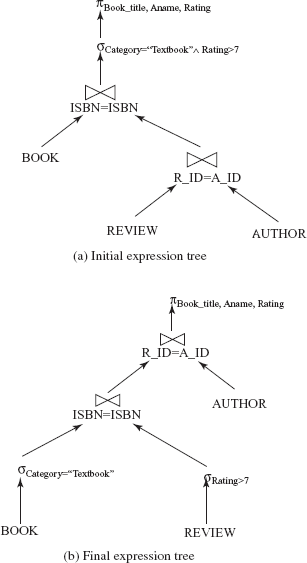
Fig. 8.14 An example of performing multiple transformations

Therefore, the project operation can be distributed over the join using rule 9(a). Moreover, the only attribute involved in join operation is P_ID of both the relations. Thus, rule 9(b) can also be applied on this expression in order to further reduce the size of the intermediate relation. The expression now becomes

ΠBook_title, Pname((ΠBook_title,P _ ID(BOOK)) (ΠP _ ID, Pname(PUBLISHER)))

It is clear from this example that the extraneous attributes can be eliminated before applying join or select operations to reduce the size of intermediate relation.

Join Ordering

Another way to reduce the size of intermediate results is to choose an optimal ordering of join operations. Thus, most of the query optimizers pay a lot of attention to the proper ordering of join operations. As discussed earlier, the join operation is commutative and associative in nature. That is,

R1 R2 = R2 R1

(R1 R2) R3 = R1 (R2 R3)

Though the expressions on the left-hand side and right-hand side in the second equation are equivalent, the cost of evaluating these two expressions may be different. Thus, it is the responsibility of the query optimizer to choose an optimal join order with the minimal cost. For example, consider a join operation on three relations R1, R2, and R3.

R1 R2 = R3

Since the join operation is associative and commutative in nature, these three relations can be joined in 12 different ways as given here.

R1(R2 R3) R1 (R3 R2) (R2 R3) R1(R3 R2) R1

R2(R1 R3) R2 (R3 R1) (R1 R3) R2 (R3 R1) R2

R3(R1 R2) R3 (R2 R1) (R1 R2) R3(R2 R1) R3

In general, for n relations, there are (2(n–1))!/(n–1)! different join orderings. For example, for n=5, the join orderings are 1680, for n = 6, the join orderings are 30240. As n increases, the number of join orderings also increases manifolds. However, generating such a large number of equivalent expressions for a given expression is not feasible.

The query optimizer, therefore, generates only a subset of equivalent expressions. For example, for the join operation (R1 R2 R3) R4 R5, it is not necessary to generate 1680 expressions. First the different join orders of R1 R2 R3 are generated and the best join order with the least cost can be found. Then, the resultant intermediate relation say, Ri generated from the join of relations {R1, R2, R3} is joined with the remaining two relations, that is, Ri R4 R5. Thus, instead of 1680 expressions, only 12 +12=24 expressions need to be examined.

In addition to finding the optimal join ordering, it is also necessary to find the order in which the tuples are generated by the join of several relations as it may affect the cost of further joins. If any particular sorted order of the tuples is useful for some operation later on, it is known as interesting sort order. For example, generating the tuples of R1 R2 R3 sorted on the attribute common with R4 or R5 is more useful than generating tuples sorted on the attributes common to only R1 and R2. Thus, the goal is to find the best join order for each subset, for each interesting sort order of the join result for that subset.

To understand the need of proper join ordering, consider the query “Retrieve the publisher name, rating, and the name of the authors who have rated the C++ book”. The corresponding relation algebra expression for this query is

ΠPname,Rating,Aname((σBook_title=“C++”(BOOK)) PUBLISHERREVIEWAUTHOR))

In this query, first the selection is performed on the BOOK relation. This will generate a set of tuples with book title C++. If the operation PUBLISHERREVIEW is performed first, it results in the Cartesian product of these two relations as no common attributes exist between PUBLISHER and REVIEW, which results in a large intermediate relation. As a result, this strategy is rejected. Similarly, the operation PUBLISHERAUTHOR is also rejected for the same reason.

If the operation REVIEWAUTHOR is performed, it also results in a large intermediate relation but the user is only interested in the authors who have reviewed the C++ book. Thus, this order of evaluating join operation is also rejected. However, if the result obtained after the select operation on BOOK relation is joined with the PUBLISHER, which in turn joined with REVIEW relation, and finally with the AUTHOR relation, the number of tuples is reduced as shown in Figure 8.15. Thus, the equivalent final expression is

ΠPname,Rating,Aname((((σBook_title=“C++”(BOOK)PUBLISHER)REVIEW) AUTHOR))

Fig. 8.15 An example of join ordering

Converting Query Trees into Query-Evaluation Plans

Generating only a set of logically equivalent expressions is not enough. A query-evaluation plan is also needed that defines exactly which algorithm should be used for each operation in the query. A query-evaluation plan can be generated by annotating each operation in the query tree with the instructions that specify the algorithm to be used to evaluate the operation. Since each relational algebra operation can be implemented with different algorithms (discussed in Section 8.3), a number of query-evaluation plans can be generated. One such possible query-evaluation plan for the expression given in Figure 8.14(b) is given in Figure 8.16.

Estimating Statistics

The statistics are used to estimate the size of intermediate results. Some of the statistics about database relations is stored in DBMS catalog, which include:

• the number of tuples in relation R, denoted by nR.
• the number of blocks containing the tuples of relation R, denoted by bR.
• the blocking factor of relation R, denoted by fR is the number of tuples that fit in one block.
• the size of each tuple of relation R in bytes, denoted by sR.
• the number of distinct values appearing in relation R for the attribute A, denoted by V(A,R). This value is same as the size of ΠA (R). If A is a key attribute, then V(A,R) = nR.
• height of index i, that is, number of levels in i, denoted by H_i.

Fig. 8.16 Query-evaluation plan

Assuming that the tuples of relation R are stored together physically in a file, then

bR = nR/fR

Every time a relation is modified, the statistics must also be updated. Updating the statistics incurs a substantial amount of overhead, thus, most of the systems update the statistics in the period of light system load—rather than updating it on every update.

In addition to the relation sizes and indexes height, real-world query optimizers also maintain some other statistical information to increase the accuracy of cost estimates. For example, most databases maintain histograms representing the distribution of values for each attribute. The values for the attribute are divided into a number of ranges, and the number of tuples whose attribute value falls in a particular range is associated with that range in the histogram. For example, the histograms for the attributes Price and Page_count of the BOOK relation are shown in Figure 8.17.

A histogram takes very little space so histograms on various attributes can be maintained in the system catalog. A histogram can be of two types, namely, equi-width histogram and equi-depth histogram. In equi-width histograms, the range of values is divided into equal-sized subranges. On the other hand, in equi-depth histograms, the sub ranges are chosen in such a way that the number of tuples within each sub range is equal.

Size Estimation for Select Operations The estimated size (number of tuples returned) of the result of a select operation depends on the selection condition.

Fig. 8.17 Histograms on Price and Page_count

• For the select operation of the form σA=a (R), the result can be estimated to have nR/V(A,R) tuples, assuming that the values are distributed uniformly (that is, each value appears with equal probability). For example, consider a relational algebra expression σPage _ count=200(BOOK). The BOOK relation contains 9 tuples (nR) and number of distinct values for the attribute Page_count [V(A,R)] is 6 (that is, 200, 450, 800, 500, 650, 550). Therefore, the result of this select operation is estimated to have 9/6 = 1.5 tuples.

  Note that the assumption that the values are distributed uniformly is not always true as it is unrealistic to assume that each value appears with equal probability. However, despite the fact that the uniform-distribution assumption is generally not correct, this method provides good approximation in many cases and keeps our presentation relatively simple.

  If a histogram is available for the attribute A, the number of tuples can be estimated with more accuracy. The range in which the value a belongs is first located in the histogram. The variable nR is replaced with the frequency count and V(A,R) is replaced with the number of distinct values appearing in that range. For example, the histogram for the attribute Page_count shows that the select operation σPage _ count=200(BOOK) is estimated to have 3/1 = 3 tuples because the frequency for the range 1–200 is 3 and the number of distinct values appearing in this range is only 1 (that is, 200).

• For the select operation of the form σA<=a(R), the estimated number of tuples that will satisfy the condition A < = a is 0 if a<min(A,R), is nR if a> = max(A,R) and
  

  otherwise. Here, min(A,R) and max(A,R) is the minimum and maximum values for the attribute A. These values can be stored in the catalog. In this case also, if a histogram is available, more accurate estimate can be obtained.

• For the select operation of the form σA>a(R) the result can be estimated to have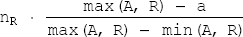
  

  tuples.

• For the conjunctive selection of the form σc1^ c2^ … ^ cn(R), the size si of each selection condition ci can be estimated as described earlier. Thus, the probability that a tuple satisfies selection condition ci is si/nR. This probability is called the selectivity of the selection σci(R). Therefore, the number of tuples in the complete conjunctive selection is
  

  where, the term

  

  represents the probability that a tuple satisfies all the conditions. It is simply the product of all the probabilities (assuming that the conditions are independent of each other).

• For the disjunctive selection of the form σc1 ∨ c2 ∨ … ∨ cn(R), the probability that a tuple satisfies all the disjunction conditions is 1 minus the probability that it will satisfy none of the conditions. That is,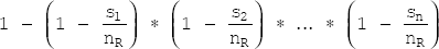
  

  The number of tuples in the complete disjunctive selection is estimated by using the following equation.

  
• For the negation selection of the form σ¬c(R), the estimated number of tuples in the absence of null values is

   

  nR – size(σc(R))

  If null values are accounted, then the estimated number of tuples can be calculated by first estimating the number of tuples for which the condition c would evaluate to unknown. This number is then subtracted from the estimate calculated earlier that ignore null values.

Size Estimation for Join Operations Estimating the size of a natural join operation is more complicated than that of the selection operation. Let RA and SA denote all the attributes of relation R and S, respectively.

• If RA ∩ SA = ϕ, that is, the relations have no common attributes, then the size estimate of the operation R S is same as that of R X S.
• If RA ∩ SA forms the key of R and foreign key of relation S, then the number of tuples returned by the operation R S is exactly the same as the number of tuples in S, that is, nS. However, if RA ∩ SA forms the key of S and foreign key of relation R, then the number of tuples returned by the operation R S is exactly the same as the number of tuples in R, that is, nR.
• If RA ∩ SA neither forms the key of R nor S, the size estimate is most difficult to find. Assuming that each value appears with equal probability, the estimated number of tuples produced by a tuple t of R in R S is
  

Therefore, the estimated number of tuples produced by all the tuples of R in R S is

If the roles of both the relations are reversed in the preceding estimate, the size estimate becomes

If V(A,R) ≠ V(A,S), then the cost estimates of both the equations differ. Then the lower value of the two estimates obtained is probably the more accurate one. If histograms are available on the join attributes, more accurate estimate can be obtained.

For example, consider a join operation BOOKPUBLISHER. Since the attribute P_ID of PUBLISHER relation is the foreign key in the BOOK relation, then the number of tuples obtained is exactly nBOOK, which is 5000.

Size Estimation for Project Operations As discussed in Chapter 04, the project operation gives result after removing duplicates. Thus, the estimated size of the project operation of the form Π_A (R) is V(A,R), where V(A,R) is the number of distinct values appearing in relation R for the attribute A. For example, the operation ΠCategory, Page_count(BOOK) returns seven tuples for the relation BOOK as shown in Figure 8.18. Since the project operation removes duplicate tuples from the resultant relation, the tuples (Textbook, 800) and (Novel, 200) appear only once in the resultant relation, though the combination of these values appears repeatedly in BOOK relation.

Size Estimation for Set Operations If the inputs to the set operations union, intersection, and set difference are the selections on the same relation say R, these set operations can be rewritten as disjunction, conjunction, and negation, respectively. For example, the set operation σc1 (R) ∪ σc2(R) can be rewritten as σc1∨c2(R) and σc1(R) ∩ σc2(R) can be rewritten as σc1∧c2(R). Since, these operations are now disjunctive and conjunctive selections, respectively, their sizes can be estimated as described earlier.

However, if the two inputs are not the selections on the same relation, the estimated size of R∪S is simply the sum of sizes of R and S, provided both the relations do not contain any common tuples. If some of the tuples are common then this estimate only gives the upper bounds on the size. Similarly, for the operation R ∩ S, the estimated size is the minimum of the sizes of R and S, provided that the smaller relation say, S contains all the tuples appearing in R. If some of the tuples of S do not appear in R then this estimate also gives the upper bound on the size. For the operation R – S, the estimated size is same as the size of R, provided no tuple of R appears in S. If some of tuples of R appear in S, then this estimate gives only the upper bound on the size.

Category	Page_count
Novel	200
Textbook	450
Textbook	800
Language Book	200
Language Book	500
Textbook	650
Textbook	550

Fig. 8.18 Result of the operation π_{Category, Page_count}(BOOK)

Size Estimation for Aggregate Operations. The estimated size of the aggregate operation of the form AF(R) is V(A,R) because for each distinct value of A, there is only one tuple returned by the aggregate operation. Here, A is the attribute of relation R on which the aggregate function F is to be applied.

NOTE The estimated statistics coupled with the cost estimates for various algorithms discussed in Section 8.3 give the estimated cost of a query-evaluation plan. The least-costly query-evaluation plan is finally chosen for the execution.

8.5.2 Heuristic Query Optimization

In cost-based optimization, generating a large number of query-evaluation plans for a given query, and finding the cost of each plan can be very time-consuming and expensive. Thus, finding the optimal plan from such a large number of plans requires a lot of computational effort. To reduce this cost and computational effort, optimizers apply some heuristics (rules) to find the optimized query-evaluation plan. These rules are known as heuristics as they usually (but not always) help in reducing the cost of execution of a query. The heuristic query optimizers simply apply these rules without finding out whether the cost is reduced by this transformation.

Generally, many different relational algebra expressions and hence, many different query trees can be created for the same query. The query parser; however, usually generates a standard initial query tree that corresponds to an SQL query without any optimization. The heuristic query optimizer then transforms this initial (canonical) query tree into the final, optimized query tree, which is more efficient to execute. However, the heuristic optimizer must make sure that the transformation steps always result in an equivalent query tree. For this, the query optimizer must be aware of the equivalence rules that preserve this equivalence. In general, the heuristic query optimizer follows these steps to transform initial query tree into an optimal query tree.

1. Conjunctive selection operations are transformed into cascading selection operations (equivalence rule 1).
2. Since the select operation is commutative with other operations according to the equivalence rules 2, 4, 8, and 11, it is moved as far down the query tree as permitted by the attributes involved in the selection condition. That is, select operation is performed as early as possible to reduce the number of tuples returned.
3. The select and join operations that are more restrictive (result in relations with the fewest tuples) are executed first. That is, the select and join operation are rearranged so that they are accomplished with the least amount of system overhead. This is done by reordering the leaf nodes of the tree among themselves by applying rule 6, 7, and 10 (commutativity and associativity of binary operations).
4. Any Cartesian product operation followed by a select operation is combined into a single join operation according to the equivalence rule 5(a).
5. The cascaded project operation is broken down and the attributes in the projection list are moved down the query tree as far as possible. New project operation can also be created as required. The attributes that are required in the query result and in the subsequent operations should only be kept after each project operation. This will eliminate the return of unnecessary attributes (rules 3, 4, 9, and 12).
6. The sub trees that represent groups of operations that can be executed by a single algorithm are identified.

To understand the use of heuristics in query optimization, consider these relational algebra expressions.

Expression 5: ΠPname,Address(σCategory=“Novel”(BOOKPUBLISHER))

The initial query tree of this expression is given in Figure 8.19(a). After applying the select operation on the BOOK relation early, the number of tuples can be reduced. Similarly, after applying the project operation to extract the desired attributes P_ID, Pname and Address from the PUBLISHER relation, and P_ID from the result of σ on BOOK relation (P_ID is the join attribute), the size of the intermediate result can be reduced further. The final expression now becomes

ΠPname,Address((ΠP_ID(σCategory=“Novel”(BOOK))) (ΠP_ID,Pname,Address(PUBLISHER)))

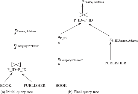
Fig. 8.19 Query trees for expression 5

The transformed query tree of the final expression after applying the select and project operations earlier is given in Figure 8.19(b).

Expression 6: ΠBook _ title,Rating(σRating>7 ∧ P_ ID=“P002”(REVIEWBOOKPUBLISHER))

The initial query tree of this expression is given in Figure 8.20(a). Since the selection condition involves conjunctive condition, it can be transformed into a cascade of select operations (heuristic rule 1). This gives a greater degree of freedom in moving the select operations down the different branches of the query tree as shown in Figure 8.20(b). In addition, after interchanging the position of PUBLISHER and REVIEW relation, the number of tuples can be further reduced as the select operation on PUBLISHER relation involves primary key which returns only one tuple (heuristic rule 3). The final expression now becomes

ΠBook_title,Rating((σP_ID=“P002”(PUBLISHER)BOOK) (σRating>7(REVIEW)))

The final query tree for this expression is given in Figure 8.20(c).

Expression 7: ΠBook_title,Pname(σBOOK.P_ID=PUBLISHER.P_ID(BOOK X PUBLISHER))

The initial query tree of this expression is given in Figure 8.21(a). Since the condition involved in select operation is the join condition, the Cartesian product can be replaced by the join operation. The final expression now becomes

ΠBook_title,Pname(BOOKBOOK.P_ID=PUBLISHER.P_ID PUBLISHER)

The final query tree after replacing the Cartesian product with the join operation is given in Figure 8.21(b).

Many real-life query optimizers have additional heuristics such as restricting the search to some particular kinds of join orders, rather than considering all join orders to further reduce the cost of optimization. For example, System R optimizer considers only those join orders in which the right operand of each join is one of the base relations R1, R2, …, Rn defined in DBMS catalog. Such join orders are called left-deep join orders and the corresponding query trees are called left-deep join trees. An example of left-deep and non-left-deep join tree is given in Figure 8.22.

Fig. 8.20

Query trees for expression 6

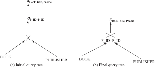
Fig. 8.21 Query trees for expression 7

The right child in left-deep trees is considered to be the inner relation when executing a nested-loop join. The main advantage of left-deep join tree is that since one of the inputs of each join is the base relation, it allows the optimizer to utilize any access path on that relation. This may speed up the execution of the join operation. Moreover, since, the right operand is always the base relation, only one input to each join needs to be pipelined. Thus, they are more convenient for pipelined evaluation.

Fig. 8.22 Left and non-left deep join trees

8.5.3 Semantic Query Optimization

Conventional query optimization techniques attempt to determine a most efficient query-evaluation plan, based on the syntax of a particular query and the access methods available. On the other hand, semantic optimization uses available semantic knowledge to transform a query into a new query which produces the same answer as the original query in any legal database state; however, requires less system resources to execute.

The semantic query optimization is a different approach that is currently the focus of considerable research. This technique operates on the key idea that the optimizer has a basic understanding of the constraints such as unique, check, and other complex constraints specified on the database schema. When a query is submitted, the optimizer uses its knowledge of system constraints to modify the given query into another query that is more efficient to execute or to simply ignore a particular query if it is guaranteed to return an empty result set. For example, consider this SQL query.

  SELECT Book_title, Page_count, Price
  FROM BOOK
  WHERE Copyright_date>Year;

This query retrieves the title, price, and page count of the books whose copyright-date is greater than the publishing year. As discussed in Chapter 03, the constraint that the copyright-date of a book is always less than its publishing year is specified on the BOOK relation. Thus, if the semantic query optimizer checks for the existence of this constraint, the query need not be executed as the query optimizer now has the knowledge that the result of the query will be empty. Hence, this technique may save a considerable time if the database catalog is checked efficiently for the constraint. However, searching the catalog for the constraints that are applicable to the given query and that may semantically optimize it can be quite time-consuming.

8.6 QUERY OPTIMIZATION IN ORACLE

In the early versions of Oracle, only rule-based query optimization was used. However, in later versions of Oracle7 and all versions of Oracle8, both rule-based and cost-based query optimizers are available. This section first discusses both types of query optimizers and then it discusses some guidelines for writing a query in Oracle.

8.6.1 Rule-based Query Optimizer

The rule-based query optimizer uses a set of 15 heuristically ranked access paths to determine the best execution plan for a query. These ranked access paths are maintained in a table, where a lower ranking implies more efficient approach and higher ranking implies lesser efficient approach. The access paths are listed in the order of their ranks in Table 8.1.

The main advantage of the rule-based optimizer is that the rule chosen is based strictly on the query structure and not on the number of tuples, partitioning or other statistics. Thus, for a given query, the execution plan is stable irrespective of the size of the relation and its related indexes. However, its main disadvantage is that the execution plan never changes despite of increase in the size of relation and its indexes.

8.6.2 Cost-based Query Optimizer

The cost-based query optimizer first generates the logically equivalent query-evaluation plans for a given query, and then determines the statistics of the relations involved in the query. These statistics are used to determine the cost of each step involved in the query-evaluation plan. Finally, the query-evaluation plan with the minimal cost is chosen for the execution of the given query. The cost-based algorithm depends entirely on the accuracy of table statistics for determining the accurate cost information. The main advantage of the cost-based optimizer is that depending on the relation and index sizes the optimizer can re-evaluate the execution plan to find the optimal execution plan.

 

Table 8.1 List of heuristically ranked access paths

Rank	Access Path
1	single row by ROWID
2	single row by cluster join
3	single row by hash cluster key with unique or primary key
4	single row by unique or primary key
5	cluster join
6	hash cluster key
7	indexed cluster key
8	composite Index
9	single column index
10	bounded range search on indexed columns
11	unbounded range search on indexed columns
12	sort–merge join
13	MAX or MIN on indexed column
14	ORDER BY indexed columns
15	complete table scan

The ANALYZE command is used for creating and maintaining the table statistics. The syntax of ANALYZE command is

  ANALYZE [TABLE <table_name> | INDEX <table_name>]
  COMPUTE STATISTICS |
  ESTIMATE STATISTICS [SAMPLE <integer> ROWS | PERCENT] |
  DELETE STATISTICS;

where,

COMPUTE STATISTICS examines all the tuples in the table to compute the exact value of statistics

ESTIMATE STATISTICS examines specified number of tuples (by default 1064 tuples) to compute the estimated size

SAMPLE is the number or percentage of rows to be used for sampling

DELETE STATISTICS deletes the statistics of the table

To understand the use of ANALYZE command, consider these examples.

• ANALYZE TABLE BOOK ESTIMATE STATISTICS SAMPLE 50 PERCENT;
• ANALYZE TABLE REVIEW COMPUTE STATISTICS;
• ANALYZE TABLE PUBLISHER ESTIMATE STATISTICS SAMPLE 1000 ROWS;
• ANALYZE TABLE BOOK DELETE STATISTICS;

NOTE The Oracle9i and later versions prefer the package DBMS_STATS instead of ANALYZE command to collect and maintain the statistics.

Once the query optimizer chooses the optimal query-execution plan, the EXPLAIN PLAN command is used to generate and store information about the plan chosen by the query optimizer. This information about the query-execution plan is stored in a table called PLAN_TABLE. Note that the EXPLAIN PLAN command gives information for SELECT, UPDATE, DELETE, and INSERT statements only.

The syntax of the EXPLAIN PLAN command is

EXPLAIN PLAN SET STATEMENT_ID = ‘<name>’

FOR <SQL statement>

where,

STATEMENT_ID is a unique ID given to every execution plan—it is just a simple string SQL statement is just a normal select statement

For example, to generate an execution plan for the query “Retrieve the title and price of all the books published by Hills Publications”, the following command can be given.

  EXPLAIN PLAN SET STATEMENT_ID =‘bookplan’
  FOR SELECT Book_title, Price
   FROM BOOK, PUBLISHER
   WHERE BOOK.P_ID=PUBLISHER.P_ID
   AND Pname=‘Hills Publications’;

This EXPLAIN PLAN statement causes the query optimizer to insert data about the execution plan for the query into PLAN_TABLE. Note that before creating a new plan with the same ID, all the entries from the PLAN_TABLE need to be deleted using the following command.

  DELETE FROM PLAN_TABLE;

8.6.3 Guidelines for Writing a Query in ORACLE

Since many different SQL statements can be used to achieve the same result, it is often the case that only one statement will be the most efficient choice in a given situation. Some guidelines are given here that give information about whether one form of the statement is more efficient than the other.

• Always include a WHERE clause in the SELECT statement to narrow the number of tuples returned until all the tuples are required. This reduces the network traffic and increases the overall performance of the query.
• Try to limit the size of the queries result set by projecting only the specific attributes (not all) from the relation.
• Try using stored procedures and views in place of large queries.
• Try using constraints in place of triggers, wherever possible.
• Try to avoid performing operations on database objects referenced in the WHERE clause. For example, consider this SQL statement.

  SELECT Book_title,Price
  FROM BOOK
  WHERE Page_count+300 > 900;

This SQL statement can be written as

  SELECT Book_title, Price
  FROM BOOK
  WHERE Page_count>600;

• Try to use the = operator as much as possible and <> operator as least as possible. This is because the <> operator slows down the execution process.
• Try to avoid the text functions such as LOWER or UPPER in the SELECT statement as it affects the overall performance. If the DBMS is case-sensitive then also avoid these text functions. For example, consider this SQL statement.

  SELECT Category
  FROM BOOK
  WHERE UPPER(Book_title) = ‘UNIX’;

  This statement can be written as

  SELECT Category
  FROM BOOK
  Book_title = ‘UNIX’ OR Book_title = ‘unix’;

• Try to avoid the HAVING clause, whenever possible as it filters the selected tuples only after all the tuples have been fetched. For example, consider this SQL statement.

  SELECT AVG(Page_count)
  FROM BOOK
  GROUP BY Category
  HAVING Category=‘Textbook’;

  This statement can be written as

  SELECT AVG(Page_count)
  FROM BOOK
  WHERE Category=‘Textbook’
  GROUP BY Category;

• Try to avoid using the DISTINCT clause, whenever possible as it results in performance degradation. It should be used only when absolutely necessary.

1. Query processing includes translation of high-level queries into low-level expressions that can be used at the physical level of the file system, query optimization, and actual execution of the query to get the result.
2. Query optimization is a process in which multiple query-execution plans for satisfying a query are examined and a most efficient query plan is identified for execution.
3. Query processing is a three-step process that consists of parsing and translation, optimization, and execution of the query submitted by the user.
4. Whenever a user submits an SQL query for execution, it is first translated into an equivalent extended relational algebra expression. During translation, the parser checks the syntax of the user’s query according to the rules of the query language. It also verifies that all the attributes and relation names specified in the query are the valid names in the schema of the database being queried.
5. The relational algebra expressions are typically represented as query trees or parse trees. A query tree is a tree data structure in which the input relations are represented as the leaf nodes and the relational algebra operations as the internal nodes.
6. To fully specify how to evaluate a query, each operation in the query tree is annotated with the instructions which specify the algorithm or the index to be used to evaluate that operation. The resultant tree structure is known as query-evaluation plan or query-execution plan or simply plan.
7. Different evaluation plans for a given query can have different costs. It is the responsibility of the query optimizer, a component of DBMS, to generate a least-costly plan. The best query-evaluation plan chosen by the query optimizer is finally submitted to the query-evaluation engine for actual execution of the query to get the desired result.
8. Whenever, a query is submitted to the database system, it is decomposed into query blocks. A query block forms a basic unit that can be translated into relational algebra expression and optimized.
9. Sorting of tuples plays an important role in database systems. If a relation entirely fits in the main memory, in-memory sorting (called internal sorting) can be performed using any standard sorting technique such as quick sort. If the relation does not fit entirely in the main memory, external sorting is required.
10. The external sort–merge algorithm is divided into two phases, namely, sort phase and merge phase.
11. The system provides a number of different algorithms for implementing several relational algebra operations such as select, join, project, set, and aggregate operations. These algorithms can be developed using indexing, iteration, or partitioning.
12. The expressions containing multiple operations are evaluated either using materialization approach or pipelining approach.
13. In materialized evaluation, each operation in the expression is evaluated one by one in an appropriate order and the result of each operation is materialized (created) in a temporary relation which becomes input for the subsequent operations.
14. With pipelined evaluation, operations form a queue and results are passed from one operation to another as they are calculated. There are two ways of executing pipelines, namely, demand-driven pipeline and producer-driven pipeline.
15. The query submitted by the user can be processed in a number of ways especially if the query is complex. It is the responsibility of the query optimizer to construct a most efficient query-evaluation plan having the minimum cost.
16. There are two main techniques of implementing query optimization, namely, cost-based optimization and heuristics-based optimization.
17. A cost-based query optimizer generates a number of query-evaluation plans from a given query using a number of equivalence rules that specify how to transform an expression into a logically equivalent one.
18. An equivalence rule states that expressions of two forms are equivalent if an expression of one form can be replaced by expression of the other form, and vice versa.
19. The cost of each evaluation plan can be estimated by collecting the statistical information about the relations such as relation sizes and available primary and secondary indexes from the DBMS catalog.
20. In addition to the relation sizes and indexes height, real-world query optimizers also maintain histograms representing the distribution of values for each attribute to increase the accuracy of cost estimates.
21. A histogram can be of two types, namely equi-width histogram and equi-depth histogram. In equi-width histograms, the range of values is divided into equal-sized sub ranges. On the other hand, in equi-depth histograms, the sub ranges are chosen in such a way that the number of tuples within each sub range is equal.
22. In cost-based optimization, generating a large number of query-evaluation plans for a given query, and finding the cost of each plan can be very time-consuming and expensive. Therefore, the optimizers use heuristic rules to reduce the cost of optimization.
23. The semantic query optimization operates on the key idea that the optimizer has a basic understanding of the constraints such as unique, check, and other complex constraints specified on the database schema.

• Query processing
• Query optimization
• Query tree (parse tree)
• Query-evaluation plan (query-execution plan)
• Query optimizer
• Query-evaluation engine
• Query block
• Internal sorting
• External sorting
• External sort–merge algorithm
• Runs
• Degree of merging
• Two-way merging
• N-way merging
• File scan
• Index scan
• Linear search (brute force)
• Binary search
• Access path
• Select operation using indexes
• Conjunctive selection
• Disjunctive selection
• Composite index
• Intersection of record pointers
• Union of record pointers
• Two-way join
• Multiway join
• Nested-loop join
• Outer relation
• Inner relation
• Result file
• Block nested-loop join
• Indexed nested-loop join
• Temporary index
• Sort–merge join
• Hybrid merge-join
• Hash join
• Partitioning phase
• Probing phase
• Skewed partitioning
• Recursive partitioning
• Hybrid hash join
• Materialized evaluation
• Operator tree
• Double buffering
• Pipelined evaluation
• Demand-driven pipeline (lazy evaluation)
• Producer-driven pipeline (eager pipelining)
• Cost-based query optimization
• Equivalence rule
• Join ordering
• Interesting sort order
• Histograms
• Equi-width histograms
• Equi-depth histograms
• Heuristic query optimization
• Left-deep join orders
• Left-deep join trees
• Semantic query optimization

A. Multiple Choice Questions

1. Which of the following DBMS components is responsible for generating a least-costly plan?
   1. Query-evaluation engine
   2. Translator
   3. Query optimizer
   4. Parser
2. If there are two relations R and S, with n and m number of tuples, respectively, the nested-loop join requires ____________ pairs of tuples to be scanned.
   1. n + m
   2. n*m
   3. m
   4. n
3. If there are two relations R and S containing 700 and 900 tuples, respectively, then which relation should be taken as outer relation in block nested-loop join algorithm?
   1. R
   2. S
   3. Any of these
   4. None of these
4. An index created by the query optimizer and destroyed when the query is completed is known as _________________.
   1. Optimized index
   2. Permanent index
   3. Temporary index
   4. Secondary index
5. Which of these is a phase in external sort–merge algorithm?
   1. Sort phase
   2. Merge phase
   3. Both (a) and (b)
   4. None of these
6. Which of these algorithms combines sort–merge join with indexes?
   1. Hybrid merge-join
   2. Indexed merge-join
   3. External merge-join
   4. Nested merge-join
7. Which of these evaluations is also known as lazy evaluation?
   1. Producer-driven pipeline
   2. Demand-driven pipeline
   3. Materialized evaluation
   4. Both (a) and (b)
8. Which of these equivalence rules is known as cascading of project operator?
   1. σc1 ∧ c2(R) = σc1(σc2(R))
   2. σc1(σc2(R)) = σc2(σc1(R))
   3. ΠA1(ΠA2(…(ΠAn(R))…)) = ΠA1(R)
   4. ΠA1,A2,…,An(σc(R)) = σc(ΠA1,A2,…,An(R))
9. Which of these operations is not commutative?
   1. Select
   2. Union
   3. Intersection
   4. Set difference
10. Given four relations P, Q, R, and S, in how many ways these relations can be joined?
    1. 4
    2. 20
    3. 16
    4. 24

B. Fill in the Blanks

1. Query processing is a three-step process that consists of parsing and translation, ___________ and execution of the query submitted by the user.
2. A __________ is a tree data structure in which the input relations are represented as the leaf nodes and the relational algebra operations as the internal nodes.
3. A ____________ forms a basic unit that can be translated into relational algebra expression and optimized.
4. The external sort–merge algorithm is divided into two phases, namely, sort phase and __________.
5. The linear search algorithm is also known as ______________ algorithm.
6. If join operation is performed on two relations, it is termed as _________________.
7. There are two main techniques of implementing query optimization, namely, _____________ optimization and _________________ optimization.
8. In _______________ histograms, the range of values is divided into equal-sized subranges.
9. A set of equivalence rules is said to be __________ if no rule can be derived from the others.
10. In ______________ pipeline, each operation at the bottom of the pipeline produces tuples without waiting for the request from the next higher-level operations.

C. Answer the Questions

1. Discuss the various steps involved in query processing with the help of a block diagram. What is the goal of query optimization? Why is it important?
2. What is a query-evaluation plan? Explain with the help of an example.
3. How does sorting of tuples play an important role in database system? Discuss the external sort–merge algorithm for select operation.
4. What are the various techniques used to develop the algorithms for relational algebra operations? Discuss the two commonly used partitioning techniques.
5. Discuss the various factors on which the cost of query optimization depends.
6. Describe the index nested loop join. How does it different from block nested loop join?
7. Compare the brute force and binary search algorithms for select operation. Which one is better?
8. Discuss the various algorithms for implementing the select operations involving complex conditions.
9. Discuss the external sort–merge algorithm for join operation.
10. Discuss the hybrid merge-join technique. How can the cost be reduced by using this technique?
11. Describe the hash join algorithm. What is the additional optimization in hybrid hash join?
12. What is recursive partitioning?
13. Discuss the algorithms for implementing various set operations.
14. Describe pipelined evaluation. Discuss its advantages over materialized evaluation. Differentiate between demand-driven and producer-driven pipelining.
15. Discuss the two techniques of optimization.
16. What is an equivalence rule? Discuss all equivalence rules.
17. Discuss the two techniques used to eliminate duplicates during project operation.
18. How does an optimal join ordering play an important role in query optimization? Explain with the help of an example. What is interesting sort order?
19. Describe the role of statistics gathered from the database in query optimization.
20. How does the available buffer size affect the result of query optimization?
21. What is a left-deep join tree? What is the significance of such a tree with respect to join pipelining?
22. How do histograms help in increasing the accuracy of cost estimates? Discuss the two types of histograms.
23. How does the heuristics help in reducing the cost of execution of a query?
24. Why do query optimizers try to apply selections early?
25. A common heuristic is to avoid the enumeration of cross products. Show a query in which this heuristic significantly reduces the optimization complexity.
26. What is meant by semantic query optimization? How does it differ from other query optimization techniques?

D. Practical Questions

1. Consider a file with 10,000 pages and three available buffer pages. Assume that the external sort–merge algorithm is used to sort the file. Calculate the initial number of runs produced in the first pass. How many passes will it take to sort the file completely? What is the total I/O cost of sorting the file? How many buffer pages are required to sort the file completely in two passes?
2. Consider three relations R(A, B, C), S(C, D, E) and T(E, F). If R has 500 tuples, S has 1000 tuples, and T has 900 tuples. Compute the size of RST, and give an efficient way for computing the join.
3. Consider the following SQL queries. Which of these queries is faster to execute and why? Draw the query tree also.
   1. SELECT Category, COUNT(*) FROM BOOK
WHERE Category!=‘Novel’
GROUP BY Category;
   2. SELECT Category, COUNT(*) FROM BOOK
GROUP BY Category
HAVING Category!=‘Novel’;
4. Consider the following relational algebra queries on Online Book database. Draw the initial query trees for each of these queries.
   1. ΠP_ID, Address, Phone(σState=“Georgia”(PUBLISHER))
   2. (σCategory=“Textbook” ∨ State=“Georgia”(BOOKBOOK.P_ID = PUBLISHER.P_IDPUBLISHER
   3. ΠBook_title,Category,Price(σAname=“Charles Smith”((BOOKBOOK.ISBN=AUTHOR_BOOK. ISBNAUTHOR_BOOK)AUTHOR_BOOK.A_ID=AUTHOR.A_ID AUTHOR)
5. Consider the following SQL queries on Online Book database.
   1. SELECT P.P_ID, Pname, Address, Phone
FROM BOOK B, PUBLISHER P
WHERE P.P_ID = B.P_ID AND Category = ‘Language Book’;
   2. SELECT ISBN, Book_title, Category, Price
FROM BOOK B, PUBLISHER P
WHERE P.P_ID = B.P_ID AND Pname=‘Bright Publications’
AND Price>30;
   3. SELECT ISBN, Book_title, Year, Page_count, Price
FROM BOOK B, AUTHOR A, AUTHOR_BOOK AB
WHERE B.ISBN = AB.ISBN AND AB.A_ID = A.A_ID
AND Aname = ‘Charles Smith’;

   4. SELECT Book_title, Pname, Aname
FROM BOOK B, PUBLISHER P, AUTHOR A, AUTHOR_BOOK AB
WHERE P.P_ID = B.P_ID AND AB.A_ID=A.A_ID
AND B.ISBN=AB.ISBN AND Category=‘Language book’;

Transform these SQL queries into relational algebra expressions. Draw the initial query trees for each of these expressions, and then derive their optimized query trees after applying heuristics on them.