CHAPTER 4
RELATIONAL ALGEBRA AND CALCULUS
After reading this chapter, the reader will understand:
- Different query languages used to extract data from the database
- Difference between relational algebra and relational calculus
- Various unary relational algebra operations like select, project, and rename
- Various binary relational algebra operations like set operations, joins, and division operation
- Various set operations like union, intersection, difference, and cartesian product operation
- Different types of joins like equijoin, natural, and outer joins (left, right, and full outer join)
- The aggregate functions that are used to perform queries, which are mathematical in nature
- Two forms of relational calculus, namely, tuple relational calculus and domain relational calculus
- The use of tuple variables for defining queries in tuple relational calculus
- Transformation of the universal and existential quantifiers
- The concept of safe expressions
- The use of domain variables for defining queries in domain relational calculus
- Expressive power of relational algebra and relational calculus
The two formal languages associated with relational model that are used to specify the basic retrieval requests are relational algebra and relational calculus. Relational algebra provides a foundation for relational model operations and is used as a basis for applying and optimizing queries in relational database management systems. It consists of basic set of operations, which can be used for carrying out basic retrieval operations. Relational calculus, on the other hand, provides declarative notations based on mathematical logic for specifying relational queries. In relational calculus, query is expressed in terms of variables and formulas on these variables. The formula in relational calculus describes the properties of the required resultant.
Relational algebra and relational calculus are logically equivalent; however, they differ on the basis of the approach they follow to retrieve data from a relation. Relational algebra uses procedural approach by providing a step-by-step procedure for carrying out a query, whereas relational calculus uses non-procedural approach as it describes the information to be retrieved without specifying the method for obtaining that information. DBMS automatically transforms these non-procedural queries into equivalent procedural queries.
This chapter discusses various operations of relational algebra. In addition, it discusses two forms of relational calculus, namely, tuple relational calculus and domain relational calculus. The chapter then concludes with the discussion on the expressive power of relational algebra and relational calculus.
4.1 RELATIONAL ALGEBRA
Relational algebra is a procedural query language that consists of a set of operations that take one or two relations as input and result into a new relation as an output. These operations are divided into two groups. One group consists of operations developed specifically for relational databases such as select, project, rename, join, and division. The other group includes the set-oriented operations such as union, intersection, difference, and cartesian product. Some of the queries, which are mathematical in nature, cannot be expressed using the basic operations of relational algebra. For such queries, additional operations like aggregate functions and grouping are used such as finding sum, average, etc. This section discusses these operations in detail.
Things to Remember
The relational closure property states that the output generated from any type of relational operation is in the form of relations only.
4.1.1 Unary Operations
The operations operating on a single relation are known as unary operations. In relational algebra, select, project, and rename are unary operations.
Select Operation
The select operation retrieves all those tuples from a relation that satisfy a specific condition. It can also be considered as a filter that displays only those tuples that satisfy a given condition. The select operation can be viewed as the horizontal subset of a relation. The Greek letter sigma (σ) is used as a select operator.
In general, the select operation is specified as
σ<selection_condition>(R)
where,
selection_condition = |
the condition on the basis of which subset of tuples is selected | |
R = |
the name of the relation |
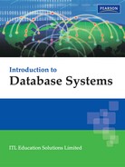
For example, to retrieve those tuples from BOOK relation whose Category is Novel, the select operation can be specified as
σCategory=“Novel”(BOOK)
The resultant relation of this operation consists of two tuples with Category as Novel and it is shown in Figure 4.1.
The comparison operators (=, ≠, <, ≤, >, ≥) can be used to specify the conditions for selecting required tuples from a relation. Moreover, more than one condition can be concatenated to one another to give a more specific condition by using any of the logical operators AND (∧), OR (∨), and NOT (¬). For example, to retrieve those tuples from BOOK relation, whose Category is Language Book and Page_count is greater than 400, the select operation can be specified as
σCategory=“Language Book” ∧ Page_count>400 (BOOK)
Consider another example, to retrieve those tuples from PUBLISHER relation, whose State is either Georgia or Hawaii, the select operation can be specified as
σState=“Georgia” ∨ State=“Hawaii” (PUBLISHER)
NOTE The comparison operators are used only with the attributes, whose domain is compatible for comparison.
The degree (number of attributes) of the relation resulting from a select operation is same as the degree of relation R. The cardinality (number of tuples) of the resulting relation is always less than or equal to the number of tuples in R.
The sequence of select operations can be applied in any order, as it is commutative in nature, that is,
σ<condition_1> (σ<condition_2> R) = σ<condition_2> (σ<condition_1> R)
In other words, the order in which conditions are applied is not significant.
Project Operation
A relation might consist of a number of attributes, which are not always required. The project operation is used to select some required attributes from a relation while discarding the other attributes. It can be viewed as the vertical subset of a relation. The Greek letter pi (π) is used as project operator.
In general, the project operation is specified as
π<attribute_list>(R)
where,
attribute_list = list of required attributes separated by commaR = the name of relation
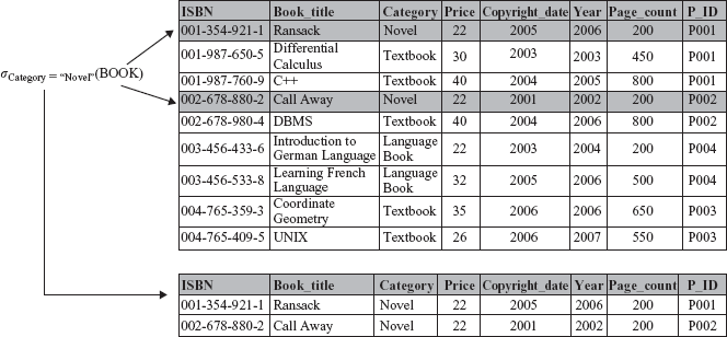
For example, to retrieve only ISBN, Book_title and Price attributes from BOOK relation, the project operation can be specified as
πISBN, Book_title, Price (BOOK)
The resultant relation of this operation consists of three attributes of all the tuples as shown in Figure 4.2.
Consider another example to retrieve P_ID, State, and Phone attributes from PUBLISHER relation, the project operation can be specified as
πP_ID, State, Phone (PUBLISHER)
The resultant relation of project operation consists of only those attributes, which are specified in <attribute_list> and are in the same order as they are appearing in the list. Hence, the degree of the resultant relation is equal to the number of attributes in <attribute_list>.
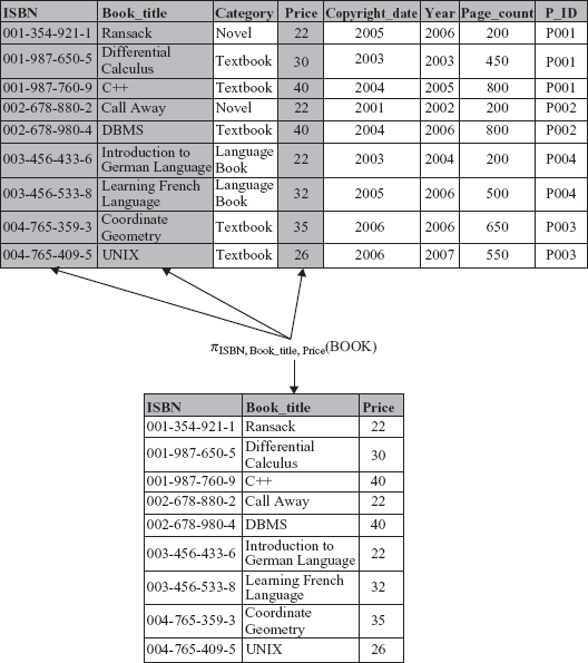
If <attribute_list> contains only non-key attributes of relation R, duplicate tuples are likely to appear in the resultant relation. The project operation removes duplicate tuples from the resultant relation. Therefore, the result of the project operation is a valid relation containing a set of unique tuples. This feature of project operation is known as duplicate elimination. For example, consider the project operation given here.
πCategory, Page_count (BOOK)
The resultant relation of this operation consists of only two attributes, namely, Category and Page_count. Since the project operation removes duplicate tuples from the resultant relation, the tuples (Textbook, 800) and (Novel, 200) appear only once in the resultant relation, although the combination of these values appear repeatedly in BOOK relation as shown in Figure 4.3.
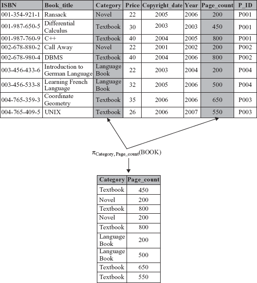
Fig. 4.3 Duplicate elimination in project operation
Unlike select operation, the commutative property does not hold on project operation, that is,
π<list_1>(π<list_2>(R)) ≠ π<list_2>(π<list_1>(R))
In other words, the order in which the list of attributes is specified in project operation is significant.
Note that, the select and project operations can also be combined together to create more complex queries. For example, to retrieve P_ID, Address, and Phone attributes from PUBLISHER relation where State is Georgia, the combined operation can be specified as
πP_ID, Address, Phone(σState=“Georgia”(PUBLISHER))
This statement first applies select operation on PUBLISHER relation and then applies project operation on the tuples retrieved from select operation.
Rename Operation
When relational algebra operations are performed, the resultant relations are unnamed, hence cannot be used for later reference. In addition, it might be required to apply more operations on the relation obtained from other operations. In such situations, rename operator proves to be useful. Rename operation is used to provide name to the relation obtained after applying any relational algebra operation. The Greek letter rho (r) is used as a rename operator. Relation obtained from any operation can be renamed by using rename operator as shown here.
ρ
(R, E)
where,
| ρ = | rename operator | |
E = |
expression representing relational algebra operations | |
R = |
name given to relation obtained by applying relational algebra operations specified in expression E |
Consider some examples of using rename operator to rename queries discussed earlier.
ρ
(R1, σCategory=“Novel”(BOOK))ρ
(R2, πP_ID, State, Phone(PUBLISHER))ρ
(R3, πP_ID, Address, Phone(σState=“Georgia”(PUBLISHER)))
Here, R1, R2, and R3 are the names given to the relations obtained from the respective relational algebra expressions. In these examples, the name of the attributes in new relation is same as in their corresponding original relations. However, attributes in a new relation can also be renamed using the rename operator as shown here.
ρ
(R(A1, A2, …An), E)
where,
A1, A2, …An are the new names provided to the attributes of the relation R, obtained after executing relational algebra expression E. For example, consider an expression given here.
ρ
(R2(P1, P2, P3), πP_ID, State, Phone(PUBLISHER))
In this example, P1, P2, P3 are new attribute names in the relation R2 for the attributes P_ID, State, and Phone of the relation PUBLISHER, respectively.
Sometimes the situation may arise where multiple relational algebra operations need to be applied in a sequence. One way to achieve this is by grouping together the sequence of operations to form a single relational algebra expression. The second way is to apply one operation at a time to create many intermediate result relations. In such situations, rename operator can be used to provide name to the intermediate relations so that they can be referred easily in the subsequent operations.
For example, consider a query to retrieve P_ID, Address, and Phone of publishers located at Georgia state. This query can be expressed in a single relational algebra expression as discussed earlier or can be expressed in two steps with the help of rename operator as shown here.
ρ
(R1, σState=“Georgia”(PUBLISHER))ρ
(R2, πP_ID, Address, Phone(R1))
In this example, select operation is applied to retrieve tuples where State is Georgia and resultant relation is named as R1. Then, the project operation is applied to retrieve selected attributes, namely, P_ID, Address, and Phone from the intermediate relation R1 and the resultant relation is named as R2. The relation R2 can further be used for more operations.
NOTE The rename operator is optional, it is not always necessary to use it. It can be used as per one’s convenience.
4.1.2 Binary Operations
The operations operating on two relations are known as binary operations. The set operations, join operations, and division operation are all binary operations.
Set Operations
The standard mathematical operations on sets, namely, union, intersection, difference, and cartesian product are also available in relational algebra. Of these, the three operations, namely, union, intersection, and difference operations require two relations to be union compatible with each other. The two relations are said to be union compatible, if they satisfy these conditions.
- The degree of both the operand relations must be same.
- The domain of nth attribute of relation
R1must be same as that of the nth attribute of relationR2.
However, the cartesian product can be defined on any two relations, that is, they need not be union compatible.
Union Operation The union operation, denoted by ∪, returns a third relation that contains tuples from both or either of the operand relations. Consider two relations R1 and R2, their union is denoted as R1 ∪ R2, which returns a relation containing tuples from both or either of the given relations. The duplicate tuples are automatically removed from the resultant relation.
For example, consider the two union compatible relations PUBLISHER_1 and PUBLISHER_2. The union of these two relations consists of tuples from both relations without any duplicate tuples as shown in Figure 4.4.

Fig. 4.4 Union operation
The union operation is, respectively, commutative and associative in nature, that is,
R1 ∪ R2 = R2 ∪ R1
and
R1 ∪ (R2 ∪ R3) = (R1 ∪ R2) ∪ R3
Intersection Operation The intersection operation, denoted by ∩, returns a third relation that contains tuples common to both the operand relations. The intersection of the relations R1 and R2 is denoted by R1 ∩ R2, which returns a relation containing tuples common to both the given relations.
For example, consider two union compatible relations PUBLISHER_1 and PUBLISHER_2. The intersection of these two relations consists of tuples common to both the relations as shown in Figure 4.5.

Fig. 4.5 Intersection operation
Like, union operation, intersection operation is, respectively, commutative and associative in nature, that is,
R1 ∩ R2 = R2 ∩ R1
and
R1 ∩ (R2 ∩ R3) = (R1 ∩ R2) ∩ R3
Learn More
Both the union and intersection operations can be performed on any number of relations, as they are associative in nature. Thus, they can be treated as n-ary operations.
Difference Operation The difference operation, denoted by − (minus), returns a third relation that contains all tuples present in one relation, which are not present in the second relation. The difference of the relations R1 and R2 is denoted by R1 − R2. The expression R1 − R2 results in a relation containing all tuples from relation R1, which are not present in relation R2. Similarly, the expression R2 − R1 results in a relation containing all tuples from relation R2, which are not present in relation R1.
For example, consider the two union compatible relations PUBLISHER_1 and PUBLISHER_2, the difference of these two relations is shown in Figure 4.6.
The difference operation is not commutative in nature, that is,
R1 − R2 ≠ R2 − R1
Note that any relational algebra expression that uses intersection operation can be rewritten by replacing the intersection operation with a pair of difference operation as shown here.
R1 ∩ R2 = R1 −(R1 − R2)

Thus, intersection operation is not a fundamental operation. It is easier to write R1 ∩ R2 than to write R1 − (R1 − R2). In addition, the intersection operation can also be expressed in terms of difference and union operations as shown here.
R1 ∩ R2 = (R1 ∪ R2) − ((R1 − R2) ∪ (R2 − R1))
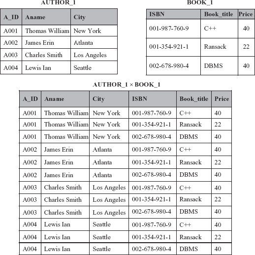
Cartesian Product Operation The cartesian product, also known as cross product or cross join, returns a third relation that contains all possible combinations of the tuples from the two operand relations. The cartesian product is denoted by the symbol ×. The cartesian product of the relations R1 and R2, is denoted by R1 × R2.
Each tuple of the first relation is concatenated with all the tuples of the second relation to form the tuples of a new relation. The cartesian product creates tuples with the combined attributes of two relations. Therefore, the degree of a new relation is the sum of the degree of both the operand relations. In addition, the cardinality of the resultant relation is the product of the cardinality of both the operand relations. In other words, if d1 and d2 are the degree of the relations R1 and R2, respectively, then the degree of the relation R1 × R2 is d1 + d2, and if c1 and c2 are the cardinality of relations R1 and R2, respectively, then the cardinality of the relation R1 × R2 is c1 * c2.
For example, consider two relations AUTHOR_1 with attributes A_ID, Aname, and City, and BOOK_1 with attributes ISBN, Book_title, and Price; the cartesian product of these two relations is shown in Figure 4.7.
In this example, each tuple from relation AUTHOR_1 is concatenated with every tuple of relation BOOK_1. The degree of both the operand relations is 3 and hence, the degree of the resultant relation is 6(3+3). The cardinality of the resultant relation is 12, which is the product of the cardinality of the relation AUTHOR_1, that is, 4 and cardinality of the relation BOOK_1, that is, 3.
NOTE The cartesian product can be made more useful and meaningful, if it is followed by select and project operations to retrieve meaningful and valuable information from the database.
Joins
The join operation is one of the most useful and commonly used operations to extract information from two or more relations. A join can be defined as a cartesian product followed by select and project operations. The result of a cartesian product is usually much larger than the result of a join.
The join operation joins two relations to form a new relation on the basis of one common attribute present in the two operand relations. That is, if both the operand relations have one common attribute defined over some common domain, then they can be joined over this common attribute. The join results in a new wider relation in which each tuple is formed by concatenating the two tuples, one from each of the operand relations, such that two tuples have the same value for that common attribute.
The join is denoted by the symbol ![]() . The most general form of the join operation is based on a condition and a pair of operand relations.
. The most general form of the join operation is based on a condition and a pair of operand relations.
That is, the join operation is specified as
R1condR2 = σcond(R1 × R2)
Note that the condition cond refers to the join condition involving attributes of both relations R1 and R2. There are different types of join operations in relational algebra, namely, equijoin, natural join, outer join, etc.
Equijoin A common case of the join operation R1 is one in which the join condition consists only of equality condition. This type of join where the only comparison operator used is, ![]() R2
R2= is known as equijoin. The resultant relation of an equijoin always has one or more pairs of attributes that have identical values in every tuple.
For example, the relations BOOK and PUBLISHER can be joined for the tuples where BOOK.P_ID is same as PUBLISHER.P_ID. This is an example of equijoin operation and it is specified as shown here.
The resultant relation of such a join is shown in Figure 4.8.

Fig. 4.8 Equijoin operation
In the resultant relation of equijoin operation, the values of the attributes PUBLISHER.P_ID and BOOK.P_ID are same for every tuple as equality condition is specified on these attributes.
The attribute publisher ID is appearing with the same name P_ID in both the relations, thus, in order to differentiate these two, the attribute names are qualified by their corresponding relation name using the dot (.) operator.
The select operation can be applied on the resultant relation to retrieve only selected tuples. For example, if only those tuples are to be displayed where the Category of book is Textbook and it is published by publishers located in Georgia, then the join operation along with the select operation can be specified as
σCategory=“Textbook” ∧ State=“Georgia”(BOOK
The result of this expression consists of a set of tuples from the resultant relation of join operation satisfying the conditions specified.
Natural Join The joins having equality condition as their join condition result in two attributes in the resulting relation having exactly the same value. However, if one of the two identical attributes is removed from the result of equijoin, it is known as natural join.
The natural join of two relations R1 and R2 is obtained by applying a project operation to the equijoin of these two relations in a sequence given here.
- Find the equijoin of two relations
R1andR2. - For each attribute
Athat is common to both relationsR1andR2, project operation is applied to remove the columnR1.AorR2.A. Therefore, if there are m attributes common in both the relations, then m duplicate columns are removed from the resultant relation of equijoin.
Learn More
Another join similar to natural join is semi-join represented as R1, is a set of all tuples from a relation ![]() R2
R2R1 having corresponding tuple in the relation R2, satisfying the join condition (equality condition). In addition, antijoin represented as R1. is a set of tuples from a relation ![]() R2
R2R1 not having corresponding tuple in the relation R2, satisfying the join condition.
The expression to obtain natural join of relations BOOK and PUBLISHER can be specified as
ISBN, Book_title, Category, BOOK.P_ID, Pname, Address, Email_ID(BOOK
The resultant relation of such a natural join is shown in Figure 4.9.
Fig. 4.9 Natural join operation
Note that, the attribute P_ID appears only once in the resultant relation of natural join. The pre-requisite of natural join is that the two attributes involved in the join condition must have the same name. If they have different names then the renaming operation is applied prior to the join operation.
Outer join The joins discussed so far are simple and are known as inner joins. An inner join selects only those tuples from both the joining relations that satisfy the joining condition. The outer join, on the other hand, selects all the tuples satisfying the join condition along with the tuples for which no tuples from the other relation satisfy the join condition.
An outer join is a type of equijoin that can be used to display all the tuples from one relation, even if there are no corresponding tuples in the second relation, thus preventing information loss. It is commonly used with relations having one-to-many relationship. The three types of outer joins are
- Left outer join: The left outer join includes all the tuples from both the relations satisfying the join condition along with all the tuples in the left relation that do not have a corresponding tuple in the right relation. The tuples from the left relation not satisfying the join condition are concatenated with the tuples having null values for all the attributes from the right relation. The left outer join of relations
R1andR2is specified asR1. condR2
 - Right outer join: The right outer join includes all the tuples from both the relations satisfying the join condition along with all the tuples in the right relation that do not have a corresponding tuple in the left relation. The tuples from the right relation not satisfying the join condition are concatenated with the tuples having null values for all the attributes from the left relation. The right outer join of relations
R1andR2is specified asR1. condR2
 - Full outer join: A full outer join combines the results of both the left and the right outer joins. The resultant relation contains all records from both the relations, with null values for the missing corresponding tuples on either side. The full outer join of relations
R1andR2is specified asR1. condR2
Division
The division operation, denoted by ÷ is useful for queries of the form ‘for all objects having all the specified properties’. To understand the division operation, consider a relation R1 having exactly two attributes A and B, and a relation R2 having just one attribute B with the same domain as in R1. The division operation R1 ÷ R2 is defined as the set of all values of attribute A, such that for every value of attribute B in R2, there is a tuple (A, B) in R1. In general, for the relations R1 and R2, R1 ÷ R2 results in the relation R3 such that R3XR2⊆R1.
For example, consider the relations R1 and R2 with the sample data as shown in Figure 4.10.
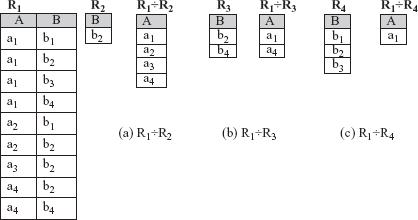
Fig. 4.10 Division operation
In this example, consider the case of division operation on the relations R1 and R2. The relation R1 ÷ R2 is the set of values that forms a tuple with every value in the relation R2, appearing in a relation R1. To elaborate further, the tuples (a1, b2), (a2, b2), (a3, b2) and (a4, b2) are appearing in the relation R1 where, b2 is a member of the relation R2 and (a1, a2, a3, a4) are members of the relation R1 ÷ R2. Similarly, the results of operations R1 ÷ R2 and R1 ÷ R4 are shown in Figure 4.10 (b) and 4.10 (c), respectively.
Now, take another example of Online Book database, ‘retrieve the list of all authors writing books for publishers located in New Jersey and Hawaii’. To achieve this, first the join operation is applied to create a relation R1(P_ID, A_ID), which contains the list of publisher ID for whom authors have written the books. Now create a relation R2(P_ID) having the list of publisher ID belonging to New Jersey or Hawaii state. The relations R1 and R2 can be obtained using these algebraic expressions.
ρ (R1, πP_ID, A_ID(BOOK
ρ (R2, πP_ID(σState=“New Jersey” OR State=“Hawaii”(PUBLISHER))
The resultant relation of division operation R1 ÷ R2 is shown in Figure 4.11.

Fig. 4.11 Example of division operation
In this example, the relation R1÷R2 is the set of values that forms a tuple with every value in relation R2, which also appears in relation R1. To elaborate further, the tuples (P002, A008) and (P003, A008) appear in the relation R1 where P002 and P003 are from relation R2.
4.1.3 Aggregate Functions and Grouping
The queries discussed so far are sufficient enough to satisfy most of the requirements of an organization. However, some of the requirements like finding total amount, average price, which are mathematical in nature cannot be expressed by basic relational algebra operations. For such type of queries, aggregate functions are used. Aggregate functions take a collection of values as input, process them, and return a single value as the result. For example, the aggregate function SUM returns a sum of the collection of numeric values taken as input. Similarly, aggregate functions, namely, AVG, MAX, and MIN are used to find average, maximum, and minimum of the collection of numeric values, respectively. The COUNT function is used for counting tuples or values in a relation.
Sometimes, situation may arise where tuples in a relation are required to be grouped, based on the values of an attribute. For example, the tuples of relation BOOK can be divided into groups based on the values of attribute Category. In other words, the books belonging to textbook category form one group, books belonging to novel category form another group, and so on.
The aggregate functions can be applied on each group individually, thus, returning a result value for each group separately. For example, for calculating average price for each category of book, AVG function is applied on each category of book separately. In other words, if there are three categories of books, then AVG function is applied to each of the three categories separately, which returns three average values for each category. The grouping of tuples of a relation can be based on one or more attributes. For example, tuples in relation BOOK can be grouped on two attributes, that is, first on the basis of category and then on the basis of publisher ID.
The aggregate function operation can be specified using the symbol ![]() (called ‘script F’) as shown here.
(called ‘script F’) as shown here.
<attribute_list><function(attribute)_list>(R)
where,
<attribute_list> = list of attributes on the basis of which tuples of a relation are to be grouped
<function(attribute)_list> = list of functions to be applied on different attributes.
For example, consider a relation BOOK, where average, maximum, and minimum price is to be calculated for each category of book separately. The expression to represent this query can be specified as
Category
The list of attributes on the basis of which tuples are grouped can be omitted from an expression. If grouping attribute is not specified in the expression, then the function is applied individually on all the tuples in the relation. Consider an example where the number of tuples in a relation has to be calculated. The required expression can be specified as
Whenever a function is applied on an attribute, the duplicate values are also included while performing the calculations. However, concatenating the function name with the string _DISTINCT can eliminate duplicate values. For example, consider a relation BOOK where the number of categories is to be calculated. If COUNT function is applied on attribute Category, it counts all the values including duplicate values. However, if COUNT_DISTINCT function is applied, it counts only the unique values.
4.1.4 Example Queries in Relational Algebra
Various operations of relational algebra can be combined together to create more advanced queries to extract required data from the database. Some of the queries are discussed here to extract information from Online Book database using operations of relational algebra.
Query 1: Retrieve city, phone and URL of the author whose name is Lewis Ian.
πCity,Phone,URL(σAname=“Lewis Ian”(AUTHOR))
In this query, the select operation is used to retrieve all the tuples where Aname is Lewis Ian, and then the project operation is used to display the required attributes, namely, City, Phone and URL for the tuples retrieved.
Query 2: Retrieve name, address, and phone of all the publishers located in New York state.
πPname, Address, Phone(σState=“New York”(PUBLISHER))
In this query, the select operation is used to retrieve all the tuples where State is New York, and then the project operation is used to display the required attributes, namely, Pname, Address, and Phone for the tuples retrieved.
Query 3: Retrieve title and price of all the textbooks with page count greater than 600.
πBook_title, Price(σCategory=“Textbook” ∧ Page_count>600(BOOK))
In this query, the select operation is used to retrieve all the tuples where Category is Textbook and Page_count is greater than 600 and then the project operation is used to display the required attributes, namely, Book_title and Price for the tuples retrieved.
Query 4: Retrieve ISBN, title, and price of the books belonging to either novel or language book category.
πISBN, Book_title, Price(σCategory=“Novel” ∨ Category=“Language Book”(BOOK))
In this query, the select operation is used to retrieve all the tuples where Category is either Textbook or Novel and then the project operation is used to display the required attributes, namely, ISBN, Book_title, and Price for the tuples retrieved.
Query 5: Retrieve ID, name, address, and phone of publishers publishing novels.
πP_ID,Pname,Address,Phone(σCategory=“Novel”(BOOK
In this query, the join of relations BOOK and PUBLISHER is created on the basis of common attribute P_ID. After creating a join, the select operation is applied on the resultant relation to retrieve all the tuples where Category is Novel, and then the project operation is used to display the required attributes, namely, P_ID, Pname, Address, and Phone for the tuples retrieved.
Query 6: Retrieve title and price of all the books published by Hills Publications.
πBook_title,Price(σPname=“Hills Publications”(BOOK
In this query, the join of relations BOOK and PUBLISHER is created on the basis of common attribute P_ID. After creating a join, the select operation is applied on the resultant relation to retrieve all the tuples where Pname is Hills Publications, and then the project operation is used to display the required attributes, namely, Book_title and Price for the tuples retrieved.
Query 7: Retrieve book title, reviewers ID, and rating of all the textbooks.
πBook_title,R_ID,Rating(σCategory=“Textbook”(BOOK
In this query, the join of relations BOOK and REVIEW is created on the basis of common attribute ISBN. After creating a join, the select operation is applied on the resultant relation to retrieve all the tuples where Category is Textbook, and then the project operation is used to display the required attributes, namely, Book_title, R_ID, and Rating for the tuples retrieved.
Query 8: Retrieve title, category, and price of all the books written by Charles Smith.
πBook_title,Category,Price(σAname=“Charles Smith” ((BOOK
In this query, the join of relations BOOK and AUTHOR_BOOK is created on the basis of common attribute ISBN and the resultant relation is joined with the relation AUTHOR on the basis of common attribute A_ID. After creating a join, the select operation is applied on the resultant relation to retrieve all the tuples where Aname is Charles Smith, and then the project operation is used to display the required attributes, namely, Book_title, Category and Price for the tuples retrieved.
Query 9: Retrieve ID, name, URL of author, and category of the book C ++.
πA_ID,Aname,URL,Category(σBook_title=“C++”((AUTHOR
In this query, the join of relations AUTHOR and AUTHOR_BOOK is created on the basis of common attribute A_ID and the resultant relation is joined with the relation BOOK on the basis of common attribute ISBN. After creating a join, the select operation is applied on the resultant relation to retrieve all the tuples where Book_title is C ++, and then the project operation is used to display the required attributes, namely, A_ID, Aname, URL, and Category for the tuples retrieved.
Query 10: Retrieve book title, price, author name, and URL for the publishers Bright Publications.
πBook_title,Price,Aname,URL(σPname=“Bright Publications”(((BOOK
In this query, four relations are joined on the basis of some common attribute. First the join of the relations BOOK and AUTHOR_BOOK is created based on the common attribute ISBN, then the resultant relation is joined with the relation AUTHOR on the basis of a common attribute A_ID. After this, the resultant relation is joined with the fourth relation PUBLISHER on the basis of a common attribute P_ID.
Finally, the select operation is applied on the resultant relation to retrieve all the tuples where Pname is Bright Publications, and then the project operation is used to display the required attributes, namely, Book_title, Price, Aname, and URL for the tuples retrieved.
Query 11: Retrieve the name and address of publishers who have not published any books.
ρ(R1, πP_ID(PUBLISHER))
ρ(R2, πP_ID(BOOK))
ρ(R3, R1 − R2)
ρ(R4, πPname, Address (R3
This query uses the difference operation to retrieve ID of publishers who have not published any books. In the first step, the list of P_ID is retrieved from the relation PUBLISHER and stored in the relation R1. In the second step, the list of P_ID is retrieved from the relation BOOK and stored in the relation R2. The relation R3 consists of a list of P_ID in the relation R1, which is not present in the relation R2. In other words, R3 stores the P_ID of the publishers having a record in relation PUBLISHER who have not published any book; hence, there is no corresponding entry in relation BOOK. Finally, after creating join of relations PUBLISHER and R3, Pname and Address for publishers who have not published any books are retrieved in relation R4.
Query 12: Retrieve the name of all the publishers and the ISBN and title of books published by them (if any).
πPname, ISBN, Book_title(BOOK
In this query, the right outer join of relations BOOK and PUBLISHER is created to retrieve the name of all the publishers and the ISBN and title of the books published by them along with those publishers who have not published any book. In that case, the values for attributes ISBN and Book_title will have null values in the resultant relation.
Query 13: Retrieve ID and the number of books written by each author.
A_ID
In this query, firstly the tuples of relation AUTHOR_BOOK are grouped on the basis of A_ID and then, the aggregate function COUNT is used to count the number of occurrences of ISBN in each group.
Query 14: Retrieve ISBN and the average rating given to each book.
ISBN
In this query, firstly the tuples of relation REVIEW are grouped on the basis of ISBN and then the aggregate function AVG is used to find the average rating in each group.
Query 15: Retrieve the name of the publishers who have published all categories of books.
ρ(R1, π Pname, Category (BOOK
ρ(R2, π Category (BOOK))
ρ(R3, R1÷R2)
In this query, firstly the join of relations BOOK and PUBLISHER is created and Pname and Category are retrieved in a relation R1. Then the unique values for Category are retrieved from the BOOK relation in another relation R2. Finally, the relation R1 is divided by the relation R2 to retrieve the name of all those publishers who have published the books of all categories in the relation R3.
4.2 RELATIONAL CALCULUS
Relational calculus, an alternative to relational algebra, is a non-procedural or declarative query language as it specifies what is to be retrieved rather than how to retrieve it. In relational calculus, queries are expressed in the form of variables and formulas consisting of these variables. The formula specifies the properties of the resultant relation without giving specific procedure for evaluating it. There are two forms of relational calculus, namely, tuple relational calculus (TRC) and domain relational calculus (DRC). In tuple relational calculus, the variable ranges over tuples from a specified relation and in domain relational calculus, the variable ranges over attributes from a specified relation. The Structured Query Language (SQL) is influenced by TRC; however, the Query-By-Example (QBE) is influenced by DRC.
4.2.1 Tuple Relational Calculus
The tuple relational calculus is based on tuple variables, which takes tuples of a specific relation as its values. A simple tuple relational calculus query is of the form
{T|P(T)}
where, T is a tuple variable and P(T) is a condition or formula for retrieving required tuples from a relation. The resultant relation of this query is the set of all tuples T for which the condition P(T) evaluates to true. For example, the query to retrieve all books having price greater than $30 can be specified in the form of tuple calculus expression as
{T | BOOK(T) ∧ T.Price>30}
The condition BOOK(T) specifies that the tuple variable T is defined for the relation BOOK. The query retrieves the set of all the tuples T satisfying the condition T.Price>30. Note that T.Price refers to the attribute Price of tuple variable T. This query extracts all the attributes of the relation BOOK. However, if only selected attributes have to be retrieved, then the attribute list can be specified in the tuple calculus expression as
{T.ISBN, T.Book_title, T.Price | BOOK(T) ∧ T.Price>30}
This expression extracts only three attributes, namely, ISBN, Book_title, and Price of the tuple set satisfying the given condition.
The tuple calculus expression consists basically of three components, which are
- The relation
Rfor which tuple variableTis defined - A condition
P(T)on the basis of which set of tuples is to be retrieved. - An attribute list specifying the required attributes to be retrieved for the tuples satisfying the given condition.
Expressions and Formulas in Tuple Relational Calculus
A general expression of the tuple relational calculus consists of a tuple variable T and a formula P(T). A formula can consist of more than one tuple variable. A formula is made up of atoms and atoms can be of any of the forms given here.
R(T), whereTis a tuple variable andRis a relation.T1.A1 opr T2.A2, whereopris a comparison operator (=,≠,<,≤,>,≥),T1andT2are tuple variables.A1is an attribute of the relation on whichT1ranges andA2is an attribute of the relation on whichT2ranges.T.A opr corc opr T.A, whereopris any comparison operator,Tis a tuple variable,Ais an attribute of the relation on whichTranges, andcis a constant in the domain of attributeA.
Each of the atoms evaluates to either true or false for a specific combination of tuples known as the truth value of an atom. A formula is built from one or more atoms concatenated with the help of the logical operators (¬, ∧,∨) by using these rules
- An atom is a formula.
- If
Fis a formula, then so is¬F. - If
F1andF2are formulae, then so areF1 ∧F2,F1∨F2 andF1⇒F2, whereF1⇒F2is also equivalent to (¬(F1) ∨F2). - If
Fis a formula, then so is ∃T(F), whereTis a tuple variable. - If
Fis a formula, then so is ∀T(F), whereTis a tuple variable.
Note that in the last two clauses, special symbols called quantifiers, namely, existential quantifier (∃) and universal quantifier (∀) are used to quantify the tuple variable T. The expression, ∀T, means ‘for every occurrence of T’ and the expression ∃T, means ‘for some occurrence of T’. A tuple variable T is said to be bound, if it is quantified, that is, it appears in (∃T) or (∀T) clause, otherwise, it is free. A tuple variable T can be said to be free or bound in a formula, on the basis of the rules given here.
- A tuple variable
Tis free in a formulaF, which is an atom. - A tuple variable
Tis free or bound in a formula of the forms(F1 ∧ F2),(F1 ∨ F2)and¬Fdepending on whether it is free or bound inF1orF2(if it occurs in either of the formulas). Note that in a formula of the formF=(F1 ∨ F2), a tuple variable may be free inF1and bound inF2, or vice versa. In such cases, one occurrence of the tuple variable is bound and the other is free inF. - All free occurrences of a tuple variable
TinFare bound in a formulaF′of the formF′ = (∃T) (F)orF′ =(∀T)(F). The tuple variable is bound to the quantifier specified inF′.
A query can be evaluated on the basis of a given instance of the database. The truth value of a formula can be derived as given here.
- An atom (formula) is true if tuple variable
Tis assigned a tuple from a relationR, otherwise it is false. ¬Fis true ifFis false, and it is false ifFis true.F1∧F2is true if bothF1andF2are true, otherwise it is false.F1∨F2is false if bothF1andF2are false, otherwise it is true.- In
F1 ⇒ F2,F2is true wheneverF1is true, otherwise it is false. (∃T)(F)is true ifFis true for some (at least one) tuple assigned to free occurrences ofTinF, otherwise it is false.(∀T)(F)is true ifFis true for every tuple (universal) assigned to free occurrences ofTinF, otherwise it is false.
Transforming the Universal and Existential Quantifiers
An expression containing a universal quantifier can be transformed into an equivalent expression containing an existential quantifier and vice versa. The steps to perform this type of transformation are
- Replace one type of quantifier into the other and precede the quantifier by NOT (¬) operator.
- Replace AND(∧) with OR(∨) operator and vice versa.
- Formula is preceded by NOT (¬) operator, as a result negated formula becomes affirmed and vice versa.
Things to Remember
In a formula, when multiple tuple variables are quantified, the evaluation takes place from inside to outside. For example, in the formula ∃T∀S(F), first ∀S will evaluate and then ∃T will be evaluated. The sequence of identical quantifiers can be altered with no other type of quantifier appearing in between.
Consider some examples of this transformation given here.
(∃T)(F) ≡ ¬(∀T)(¬F)
(∀T)(F) ≡ ¬(∃T)(¬F)
(∃T)(F1∧F2) ≡ ¬(∀T)(¬F1∨¬F2)
(∀T)(F1∨F2) ≡ ¬(∃T)(¬F1∧¬F2)
(∃T)(¬F1∨¬F2) ≡ ¬(∀T)(F1∧F2)
(∀T)(¬F1∧¬F2) ≡ ¬(∃T)(F1∨F2)
Note that the symbol ≡ represents equivalent to.
Example Queries in Tuple Relational Calculus
The queries expressed in relational algebra can also be expressed in tuple relational calculus. The difference is only in the notation used to express the queries. The queries discussed in relational algebra can be expressed in tuple relational calculus as shown here.
Query 1: Retrieve city, phone, and URL of the author whose name is Lewis Ian.
{T.City, T.Phone, T.URL | AUTHOR(T) ∧ T.Aname=“Lewis Ian”}
In this query, tuple variable T for the relation AUTHOR and the condition to retrieve required tuples from this relation is specified after the bar (|). The tuples satisfying the given condition are assigned to T, and the attribute values for City, Phone, and URL are displayed for the tuples retrieved.
Query 2: Retrieve name, address, and phone of all the publishers located in New York state.
{T.Pname, T.Address, T.Phone | PUBLISHER(T) ∧ T.State=“New York”}
In this query, the tuple variable T for the relation PUBLISHER is defined, and the tuples satisfying the given condition are assigned to T. Then, the attribute values for Pname, Address, and Phone are displayed for the tuples retrieved.
Query 3: Retrieve title and price of all the textbooks with page count greater than 600.
{T.Book_title, T.Price | BOOK(T) ∧ T.Category=“Textbook” ∧ T.Page_count>600}
In this query, the tuple variable T for the relation BOOK is defined, and the tuples satisfying the given condition are assigned to T. Then, the attribute values for Book_title and Price are displayed for the tuples retrieved.
Query 4: Retrieve ISBN, title and price of the books belonging to either novel or language book category.
{T.ISBN, T.Book_title, T.Price | BOOK(T) ∧ (T.Category=“Novel” ∨ T.Category=“Language Book”)}
In this query, the tuple variable T for the relation BOOK is defined, and the tuples satisfying the given condition are assigned to T. Then, the attribute values for ISBN, Book_title, and Price are displayed for the tuples retrieved.
Query 5: Retrieve ID, name, address, and phone of publishers publishing novels.
{T.P_ID, T.Pname, T.Address, T.Phone | PUBLISHER(T) ∧ (∃S)(BOOK(S) ∧ S.P_ID=T.P_ID ∧ S.Category=“Novel”)}
In this query, tuple variables T and S for the relations PUBLISHER and BOOK, respectively, are defined. Of these, T is a free tuple variable and S is bound to the existential quantifier. Note that the condition S.P_ID=T.P_ID is a join condition for PUBLISHER and BOOK relations. The attribute values of P_ID, Pname, Address, and Phone of all the tuples satisfying the specified condition are displayed.
Query 6: Retrieve title and price of all the books published by Hills Publications.
{T.Book_title, T.Price | BOOK(T) ∧ (∃S)(PUBLISHERS(S) ∧ S.P_ID =T.P_ID ∧ S.Pname = “Hills Publications”)}
In this query, the tuple variables T and S for the relations BOOK and PUBLISHER, respectively, are defined. Here, T is a free tuple variable and S is bound to the existential quantifier. The two relations are joined on the basis of common attribute P_ID. The attribute values of Book_title and Price of all the tuples satisfying the specified condition are displayed.
Query 7: Retrieve book title, reviewers ID, and rating of all the textbooks.
{T.Book_title, S.R_ID, S.Rating | BOOK(T) ∧ REVIEW(S) ∧ T.Category=“Textbook” ∧ T.ISBN = S.ISBN}
In this query, the tuple variables T and S for the relations BOOK and REVIEW, respectively, are defined. The two relations are joined on the basis of common attribute ISBN. The attribute values of Book_title, R_ID, and Rating of all the tuples satisfying the specified condition are displayed.
Query 8: Retrieve title, category, and price of all the books written by Charles Smith.
{T.Book_title, T.Category, T.Price | BOOK(T) ∧ ((∃S)(∃P)(AUTHOR(S) ∧ AUTHOR_BOOK(P) ∧ S.Aname=“Charles Smith” ∧ T.ISBN=P.ISBN ∧ P.A_ID=S.A_ID))}
In this query, the tuple variables T, S, and P for the relations BOOK, AUTHOR, and AUTHOR_BOOK, respectively, are defined. Here, T is a free tuple variable, whereas S and P are bound to the existential quantifiers. The relations BOOK and AUTHOR_BOOK are joined on the basis of common attribute ISBN and the resultant relation is joined with the relation AUTHOR on the basis of common attribute A_ID. After this, the attribute values for Book_title, Category, and Price of all the tuples where Aname is Charles Smith, are displayed.
Query 9: Retrieve ID, name, URL of author, and category of the book C ++.
{T.A_ID, T.Aname, T.URL, S.Category | AUTHOR(T) ∧ BOOK(S) ∧ S.Book_title =“C++” ∧ ((∃P)(AUTHOR_BOOK(P) ∧ T.A_ID=P.A_ID ∧ P.ISBN=S.ISBN))}
In this query, the tuple variables T, S, and P for the relations AUTHOR, BOOK, and AUTHOR_BOOK, respectively, are defined. Here, T and S are free tuple variables whereas P is bound to the existential quantifier. The relations AUTHOR and AUTHOR_BOOK are joined on the basis of common attribute A_ID, and the resultant relation is joined with the relation BOOK on the basis of common attribute ISBN. After this, the attribute values for A_ID, Aname, URL, and Category of all the tuples where Book_title is C ++ are displayed.
Query 10: Retrieve book title, price, author name, and URL for the publishers Bright Publications.
{T.Book_title, T.Price, S.Aname, S.URL | BOOK(T) ∧ AUTHOR(S) ∧ ((∃P) (∃R)(PUBLISHER(P) ∧ AUTHOR_BOOK(R) ∧ T.ISBN=R.ISBN ∧ R.A_ID=S.A_ID ∧ T.P_ID=P.P_ID ∧ P.Pname=“Bright Publications”))}
In this query, the tuple variables T, S, P, and R for the relations BOOK, AUTHOR, PUBLISHER, and AUTHOR_BOOK, respectively, are defined. Among these, T and S are free tuple variables, whereas P and R are bound to existential quantifiers. Here, four relations are joined on the basis of some common attribute. First the join of the relations BOOK and AUTHOR_BOOK is created on the basis of the attribute ISBN, then the resultant relation is joined with the relation AUTHOR on the basis of the attribute A_ID. After this, the resultant relation is joined with the fourth relation PUBLISHER on the basis of the attribute P_ID. Finally, the attribute values for Book_title, Price, Aname, and URL of all tuples where Pname is Bright Publications, are displayed.
Query 11: Retrieve name and address of publishers who have not published any books.
{T.Pname, T.Address | PUBLISHER(T) ∧ (¬(∃S)(BOOK(S) ∧ T.P_ID=S.P_ID))}
In this query, the tuple variables T and S for the relations PUBLISHER and BOOK, respectively, are defined. Here, T is a free tuple variable, whereas S is bound to existential quantifier. Note that the negation operator (¬) is used to retrieve the tuples, which do not satisfy the join condition, that is, it retrieves the attributes Pname and Address of the publishers who have no corresponding books in relation BOOK.
This query can also be expressed by using universal quantifier instead of existential quantifier by following general transformation rules as shown here.
{T.Pname, T.Address | PUBLISHER(T) ∧ ((∀S)(¬(BOOK(S)) ∨ ¬(T.P_ID=S.P_ID)))}
Safe Expressions
An expression of tuple relational calculus containing universal quantifier, existential quantifier or negation condition may lead to a relation of infinite number of tuples. For example, consider an expression given here.
{T | ¬BOOK(T)}
This expression appears to be syntactically correct but it refers to all the tuples in the universe not belonging to BOOK relation, which are infinite in number. These types of expressions are known as unsafe expressions. Therefore, care must be taken while using quantifier symbols and negation operator in a relational calculus expression to ensure safe expressions. A safe expression is an expression, which results in a relation with finite number of tuples.
Safe expressions can be defined more precisely by introducing the concept of the domain of a tuple relational calculus expression, E. The domain of expression E, denoted by Dom(E), is the set of all values appearing either as constant values in the expression E, or appearing in any of the tuples of relations referred by E. In other words, the domain of E is the set of all values that appear as constant in E, or appear in one or more relations whose names appear in E. Therefore, the domain of the above expression includes all the values appearing in the relation BOOK. Similarly, the domain for the Query 5 includes all the values appearing in the relations BOOK and PUBLISHER. Hence, an expression E, is said to be safe if all the values appearing in the resultant relation are from the domain of E, Dom(E).
The expression {T | ¬BOOK(T)} is said to be safe if all the values appearing in the resultant relation are from the domain, Dom(BOOK). However, this expression is unsafe as the resultant relation of this expression includes all the tuples in the universe not appearing in the BOOK relation, hence not belonging to the domain Dom(BOOK). All other expressions discussed in tuple relational calculus are safe expressions.
4.2.2 The Domain Relational Calculus
The domain relational calculus is based on domain variables, which unlike tuple relational calculus, range over the values from the domain of an attribute, rather than values for an entire tuple. A simple domain relational calculus query is of the form
{T | P(T)}
where, T represents a set of domain variables (x1, x2, …, xn) that ranges over domains of attributes (A1, A2, …, An) and P represents the formula on T. Like, tuple relational calculus, formulae in domain relational calculus are built up from atoms and an atom can be of any of the forms given here.
R(x1, x2, …, xn), whereRis a relation with n attributes andx1, x2, …, xnare domain variables or domain constants for the corresponding n attributes.x1 opr x2, whereopris a comparison operator(=, ≠, <, ≤, >, ≥)andx1andx2are domain variables. Note that the domain of attributesx1andx2are compatible for comparison.x opr corc opr x, whereopris a comparison operator,xis a domain variable andcis a constant in the domain of the attribute for whichxis a domain variable.
Formulas are built from atoms by using these rules
- An atom is a formula.
- If
Fis a formula, then so is¬F. - If
F1andF2are formulae, then so areF1∧F2,F1∨F2andF1⇒F2. - If
Fis a formula, then so is ∃x(F), wherexis a domain variable. - If
Fis a formula, then so is ∀x(F), wherexis a domain variable.
Like in tuple relational calculus, atoms evaluate to either true or false for a specific set of values. In rule 1, an atom (formula) is true, if the domain variable is assigned values corresponding to a tuple of the specified relation R. Similarly, in the remaining rules, if the domain variables are assigned values that satisfy the condition, then the atom is true, otherwise it is false.
Example Queries in Domain Relational Calculus
The queries expressed in relational algebra or tuple relational calculus can also be expressed in domain relational calculus. The difference is only in the notation used to express the queries. In domain relational calculus, the queries based on the relation AUTHOR require seven domain variables a1, a2, …, a7 to range over the domain of each attribute of the relation in order. Similarly, for the relations BOOK, PUBLISHER, AUTHOR_BOOK, and REVIEW, the number of domain variables required is eight (b1, b2, …, b8), six (p1, p2, …, p6), two (c1, c2) and three (r1, r2, r3), respectively.
In domain relational calculus, the domain variables for the attributes to be displayed are specified before the bar (|) and the relations and conditions to retrieve the required tuples are specified after the bar (|). The queries discussed earlier can be expressed in domain relational calculus as shown here.
Query 1: Retrieve city, phone, and URL of the author whose name is Lewis Ian.
{a4, a6, a7 | (∃a2) (AUTHOR(a1, a2, a3, a4, a5, a6, a7) ∧ a2=“Lewis Ian”)}
The required attributes City, Phone, and URL to be displayed are specified by free domain variables a4, a6, and a7, respectively, for the relation AUTHOR. Existential quantifier quantifies the variable a2 for which condition is specified.
Query 2: Retrieve name, address, and phone of all the publishers located in New York state.
{p2, p3, p5 | (∃p4) (PUBLISHER(p1, p2, p3, p4, p5, p6) ∧ p4 =“New York”)}
The required attributes Pname, Address, and Phone to be displayed are specified by free domain variables p2, p3, and p5, respectively, for the relation PUBLISHER. Existential quantifier quantifies the variable p4 for which condition is specified.
Query 3: Retrieve title and price of all the textbooks with page count greater than 600.
{b2, b4 | (∃b3) (∃b7) (BOOK(b1, b2, b3, b4, b5, b6, b7, b8) ∧ b3 =“Textbook” ∧ b7>600)}
The required attributes Book_title and Price to be displayed are specified by free domain variables b2 and b4, respectively, for the relation BOOK. Existential quantifiers quantify the variables b3 and b7 for which conditions are specified.
Query 4: Retrieve ISBN, title and price of the books belonging to either novel or language book category.
{b1, b2, b4 | (∃b3) (BOOK(b1, b2, b3, b4, b5, b6, b7, b8) ∧ (b3=“Novel” ∨ b3 =“Language Book”))}
The required attributes ISBN, Book_title, and Price to be displayed are specified by free domain variables b1, b2, and b4, respectively, for the relation BOOK. Existential quantifier quantifies the variable b3 for which conditions are specified.
Query 5: Retrieve ID, name, address, and phone of publishers publishing novels.
{p1, p2, p3, p5 | (∃b3) (∃b8) (BOOK(b1, b2, b3, b4, b5, b6, b7, b8) ∧ PUBLISHER(p1, p2, p3, p4, p5, p6) ∧ b8 = p1 ∧ b3 =“Novel”)}
The required attributes P_ID, Pname, Address, and Phone to be displayed are specified by free domain variables p1, p2, p3, and p5, respectively, for the relation PUBLISHER. Existential quantifiers quantify the variables b3 and b8 for which conditions are specified. The variable p1 appearing in a condition is not quantified as it is appearing as a free domain variable before the bar (|).
Note that the condition b8 = p1 is a join condition as it relates two domain variables ranging over common attributes from two different relations. This condition creates join of two relations BOOK and PUBLISHER.
Query 6: Retrieve title and price of all the books published by Hills Publications.
{b2, b4 | (∃p2) (∃p1) (∃b8) (BOOK(b1, b2, b3, b4, b5, b6, b7, b8) ∧ PUBLISHER (p1, p2, p3, p4, p5, p6) ∧ p1 =b8 ∧ p2 =“Hills Publications”)}
The required attributes Book_title and Price to be displayed are specified by free domain variables b2 and b4, respectively, for the relation BOOK. Existential quantifiers quantify the variables p2, p1, and b8 for which conditions are specified. Note that the condition p1 = b8 is a join condition as it creates a join of two relations PUBLISHER and BOOK.
Query 7: Retrieve book title, reviewers ID, and rating of all the textbooks.
{b2, r1, r3 | (∃b3) (∃b1) (∃r2) (BOOK(b1, b2, b3, b4, b5, b6, b7, b8) ∧ REVIEW(r1, r2, r3)∧ b1 =r2 ∧ b3 =“Textbook”)}
The required attributes Book_title, R_ID, and Rating to be displayed are specified by free domain variables b2 for the relation BOOK, r1 and r3 for the relation REVIEW, respectively. Existential quantifiers quantify the variables b3, b1, and r2 for which conditions are specified. Note that, the condition b1 = r2 is a join condition as it creates a join of two relations BOOK and REVIEW.
Query 8: Retrieve title, category, and price of all the books written by Charles Smith.
{b2, b3, b4 | (∃b1) (∃c2) (∃c1) (∃a1) (∃a2) (BOOK(b1, b2, b3, b4, b5, b6, b7, b8) ∧ AUTHOR(a1, a2, a3, a4, a5, a6, a7) ∧ AUTHOR_BOOK(c1, c2) ∧ b1 = c2 ∧ c1 = a1 ∧ a2 =“Charles Smith”)}
The required attributes Book_title, Category, and Price to be displayed are specified by free domain variables b2, b3, and b4, respectively, for the relation BOOK. Existential quantifiers quantify the variables b1, c2, c1, a1, and a2 for which conditions are specified. The conditions b1 =c2 and c1 =a1 creates a join of relations BOOK, AUTHOR_BOOK, and AUTHOR.
Query 9: Retrieve ID, name, URL of author, and category of the book C++.
{a1, a2, a7, b3 | (∃c1) (∃b1) (∃c2) (∃b2) (BOOK(b1, b2, b3, b4, b5, b6, b7, b8) ∧ 2 =“C++”)}
The required attributes A_ID, Aname, URL, and Category to be displayed are specified by free domain variables a1, a2, a7 for the relation AUTHOR and b3 for the relation BOOK, respectively. Existential quantifiers quantify the variables c1, b1, c2, and b2 for which conditions are specified. Note that variable a1 appearing in a condition is not quantified as it is appearing as free domain variable before the bar (|). The conditions a1 = c1 and c2 = b1 creates a join of relations AUTHOR, AUTHOR_BOOK, and BOOK.
Query 10: Retrieve book title, price, author name, and URL for the publishers Bright Publications.
{b2, b4, a2, a7 | (∃a1) (∃c1) (∃c2) (∃b1) (∃b8) (∃p1) (∃p2) (BOOK(b1, b2, b3, b4, b5, b6, b7, b8 ∧ AUTHOR(a1, a2, a3, a4, a5, a6, a7) ∧ AUTHOR_BOOK (c1, c2) ∧ PUBLISHER(p1, p2, p3, p4, p5, p6) ∧ a1 =c1 ∧ c2 =b1 ∧ b8 =p1 ∧ p2 = “Bright Publications”)}
The required attributes Book_title, Price, Aname, and URL to be displayed are specified by free domain variables b2, b4 for the relation BOOK and a2, a7 for the relation AUTHOR, respectively. Existential quantifiers quantify the variables a1, c1, c2, b1, b8, p1, and p2 for which conditions are specified. The conditions a1 =c1, c2 =b1, and creates a join of relations b8 = p1AUTHOR, AUTHOR_BOOK, BOOK, and PUBLISHER.
Query 11: Retrieve name and address of publishers who have not published any books.
{p2, p3 | (∃p1) (PUBLISHER(p1, p2, p3, p4, p5, p6) ∧ (¬(∃b8) (BOOK(b1, b2, b3, b4, b5, b6, b7, b8) ∧ p1 =b8)))}
The required attributes Pname and Address to be displayed are specified by free domain variables p2, and p3, respectively for the relation PUBLISHER. Existential quantifiers quantify the variables p1 and b8 for which conditions are specified. The negation operator (¬) is used to retrieve those publisher IDs who have not published any book.
This query can also be expressed by using universal quantifier instead of existential quantifier by following general transformation rules as shown here.
{p2, p3 | (∃p1) (PUBLISHER(p1, p2, p3, p4, p5, p6) ∧ ((∀b7) (¬(BOOK(b1, b2, b3, b4, b5, b6, b7, b8)) ∨ ¬(p1=b7))))}
4.3 EXPRESSIVE POWER OF RELATIONAL ALGEBRA AND RELATIONAL CALCULUS
As discussed earlier, the relational algebra provides a procedure for solving a problem, whereas relational calculus simply describes what the requirement is. However, relational algebra and relational calculus are logically equivalent. That is, for every safe relational calculus expression there exists equivalent relational algebra expression and vice versa. In other words, there is one-to-one mapping between the two and the difference lies only in the way the query is expressed.
The expressive power of relational algebra is frequently used as a metric to measure the power of any relational database query language. A query language is said to be relationally complete if it is at least as powerful as relational algebra, that is, if it can express any query expressed in relational algebra. Relational completeness has become an important basis for comparing the expressive power of various relational database query languages. Most of the relational database query languages are relationally complete. In addition, they have more expressive power than relational algebra or relational calculus with the inclusion of various advanced operations such as aggregate functions, grouping, and ordering.
SUMMARY
- Relational algebra is a procedural query language that consists of a set of operations that take one or two relations as input, and result into a new relation as an output.
- Relational algebra operations are divided into two groups. One group consists of operations developed specifically for relational databases such as select, project, rename, join, and division. The other group includes the set-oriented operations such as union, intersection, difference, and cartesian product.
- The select operation retrieves all those tuples from a relation that satisfy a specific condition. The Greek letter sigma (σ) is used as a select operator.
- The project operation is used to select some required attributes from a relation while discarding the other attributes. The Greek letter pi (π) is used as project operator.
- Rename operation is used to provide name to the relation obtained after applying any relational algebra operation. The Greek letter rho (ρ) is used as a rename operator.
- The union operation, denoted by ∪, returns a third relation that contains tuples from both or either of the operand relations.
- The intersection operation, denoted by ∩, returns a third relation that contains tuples common to both the operand relations.
- The difference operation, denoted by
−(minus), returns a third relation that contains all tuples present in one relation, which are not present in the second relation. - The cartesian product, also known as cross product or cross join, returns a third relation that contains all possible combinations of the tuples from the two operand relations. The cartesian product is denoted by the symbol
×. - A join can be defined as a cartesian product followed by select and project operations. The join operation joins two relations to form a new relation on the basis of one common attribute present in the two operand relations.
- A common case of the join operation in which the join condition consists only of equality condition is known as equijoin.
- The equijoin operation results in two attributes in the resulting relation having exactly the same value. If one of the two identical attributes is removed from the result of equijoin, it is known as natural join.
- An inner join selects only those tuples from both the joining relations that satisfy the joining condition. The outer join, on the other hand, selects all the tuples satisfying the join condition along with the tuples for which no tuples from the other relation satisfy the join condition.
- There are three types of outer joins, namely, left outer join, right outer join, and full outer join.
- Some of the requirements like finding total amount, average price, which are mathematical in nature, cannot be expressed by basic relational algebra operations. For such type of queries, aggregate functions are used. Aggregate functions take a collection of values as input, process them, and return a single value as the result.
- Relational calculus, an alternative to relational algebra, is a non-procedural or declarative query language as it specifies what is to be retrieved rather than how to retrieve it. In relational calculus, queries are expressed in the form of variables and formulas consisting of these variables.
- There are two forms of relational calculus, namely, tuple relational calculus (TRC) and domain relational calculus (DRC).
- The tuple relational calculus is based on tuple variables, which takes tuples of a specific relation as its values.
- An expression of tuple relational calculus containing universal quantifier, existential quantifier or negation condition may lead to a relation of infinite number of tuples. These types of expressions are known as unsafe expressions. A safe expression, on the other hand, results in a relation with finite number of tuples.
- The domain relational calculus is based on domain variables, which unlike tuple relational calculus, range over the values from the domain of an attribute, rather than values for an entire tuple.
- The expressive power of relational algebra is frequently used as a metric to measure the power of any relational database query language. A query language is said to be relationally complete if it is at least as powerful as relational algebra, that is, if it can express any query expressed in relational algebra.
KEY TERMS
- Select operation
- Project operation
- Rename operation
- Union operation
- Intersection operation
- Difference operation
- Cartesian product
- Join operation
- Equijoin
- Natural join
- Outer join
- Left outer join
- Right outer join
- Full outer join
- Division
- Aggregate functions
- Tuple relational calculus
- Tuple variable
- Atom
- Formula
- Existential quantifier
- Universal quantifier
- Safe expression
- Domain relational calculus
- Domain variable
EXERCISES
A. Multiple Choice Questions
- Which of the following is the operation developed specifically for the relational databases?
- Union
- Cartesian product
- Division
- Difference
- Which of the following is the set-oriented operation?
- Select
- Difference
- Division
- Project
- Which of the following is the binary operation?
- Union
- Join
- Cartesian product
- All of these
- Which of the following is true for right outer join?
- It includes all the tuples from both the relations satisfying the join condition along with all the tuples in the right relation that do not have a corresponding tuple in the left relation.
- It includes all the tuples from both the relations satisfying the join condition along with all the tuples in the left relation that do not have a corresponding tuple in the right relation.
- It selects all the tuples satisfying the join condition along with the tuples for which no rows from the other relation satisfy the join condition.
- None of these
- Which of the following aggregate functions is used for counting tuples or values in a relation?
AvgCountMaxMin
- Which of the following is the component of tuple calculus expression?
- The relation
Rfor which tuple variableTis defined. - A condition
P(T)on the basis of which set of tuples is to be retrieved. - An attribute list specifying the required attributes to be retrieved for the tuples satisfying the given condition.
- All of these
- The relation
- The truth value of a formula can be derived as
¬Fis true ifFis false, and it is false ifFis true.F1∧F2is true if bothF1andF1andF2are true, otherwise it is false.F1∨F1andF52are false, otherwise it is true.- All of these
- Which of the following is symbol for existential quantifier?
- ∀
- ∃
- ¬
- ≡
- Which of the following statements is true?
(∀T)(F) ≡ ¬(∃T)(F)(∃T)(F1∧F2) ≡ ¬(∀T)(¬F1∨¬F2)(∀T)(F1∨F2) ≡ (∃T)(¬F1∧¬F2)(∀T)(F1∧F2) ≡ ¬(∃T)(F1∨F2)
- Which of the following is not a rule for forming formula in domain relational calculus?
- An atom is a formula.
- If
Fis a formula, then so is ¬F. - If
F1andF2are formulae, then so areF1∧F2,F1∨F2andF1 ⇒ F2. - If
Fis a formula, then so is ∃T(F), whereTis a tuple variable.
B. Fill in the Blanks
- The _____________ is used to select some required attributes from a relation while discarding the other attributes.
- ______________ is used to provide name to the relation obtained after applying any relational algebra operation.
- The _____________ can be defined on any two relations, that is, they need not be union compatible.
- Relational algebra expression that uses intersection operation can be rewritten by replacing the intersection operation with a pair of _____________ operation.
- A common case of the join operation
R1is one in which the join condition consists only of equality condition, also known as _____________.R2 - The ________________ is useful for queries of the form ‘for all objects having all the specified properties’.
- A tuple variable
Tis said ___________, if it is quantified, that is, it appears in(∃T)or(∀T)clause, otherwise, it is __________. - A ____________ is an expression, which results in a relation with a finite number of tuples.
- The ______________ is based on domain variables, which unlike tuple relational calculus, range over the values from the domain of an attribute, rather than values for an entire tuple.
- A query language is said to be ___________ if it is at least as powerful as relational algebra, that is, if it can express any query expressed in relational algebra.
C. Answer the Questions
- Give similarities and differences between relational algebra and relational calculus.
- What are the various unary and binary operations in relational algebra? Why are they called so?
- Discuss various unary operations of relational algebra with example.
- What do you mean by union compatibility of relations? Explain with example.
- Discuss various set operations of relational algebra with example.
- What is the purpose of rename operator in relational algebra?
- What is the role of join operations in relational algebra? Differentiate between equijoin and natural join.
- What are outer join operations and how are they different from inner join operations? Discuss various types of outer join operations.
- What is cartesian product? How is it different from join operation?
- Discuss division operation in detail with example.
- What is relational calculus? What are its two forms? Differentiate between them.
- What information is required to be specified in tuple calculus expression? Explain with example.
- What are quantifiers and what are its types? How is existential quantifier transformed into universal quantifier and vice versa? Give suitable examples.
- When is an expression in tuple relational calculus said to be unsafe? How can safe expressions be defined? Explain with example.
- Differentiate between the following:
- Tuple variable and domain variable
- Atom and formula
- What are the different forms of atom in tuple relational calculus and domain relational calculus? Give rules for forming formulas in tuple relational calculus and domain relational calculus.
- Convert the following domain calculus expression into corresponding, English statement, relational algebra expression and tuple calculus expression.
{b2, r1, r3 | (∃b3) (∃b1) (∃r2) (Rel_1(b1, b1, r2, r3) ∧ b1 =r2 ∧b3=“ABC”)} - What do you understand by the expressive power of relational algebra? How are relational algebra and relational calculus logically equivalent? When is a query language said to be relationally complete?
D. Practical Questions
- 1. Consider the following relational schema for the
SALESdatabase:CUSTOMER(CustNo, CName, City) ORDER(OrderNo, OrderDate, CustNo, Amount) ORDER_ITEM(OrderNo, ItemNo, Qty) ITEM(ItemNo, UnitPrice)
On the basis of this relational schema, write the following queries in relational algebra, tuple calculus, and domain calculus.
- Retrieve number and date of orders placed by customers residing at Atlanta city.
- Retrieve number and unit price of items for which order of quantity greater than 50 is placed.
- Retrieve order number, date, and item number for the order of items having unit price greater than 20.
- Retrieve details of customers who have placed order for the item number I010.
- Retrieve number and unit price of items for which order is placed by the customer number C001.
- Given the relational schemes:
ENROL(S#, C#, Section)—S# represents student numberTEACH(Prof, C#, Section)—C# represents course numberADVISE(Prof, S#)—Prof is thesis advisor of S#PRE_REQ(C#, Pre_C#)—Pre_C# is prerequisite courseGRADES(S#, C#, Grade, Year)STUDENT(S#, Sname)—Sname is student nameExpress the following queries in relational algebra, tuple calculus, and domain calculus.
- List all students taking courses with Zeba.
- List all students taking at least one course that their advisor teaches.
- List those professors who teach more than one section of the same course.
- Consider the relational database:
EMPLOYEE(Empname, Street, City)WORKS(Empname, Companyname, Salary)COMPANY(Companyname, City)MANAGES(Empname, Managername)Give an expression in the relational algebra for each request.
- Find the names of all employees who work for First Bank Corporation.
- Find the names, street addresses, and cities of residence of all employees who work for First Bank Corporation and earn more than 200,000 per annum.
- Find the names of all employees in this database who live in the same city as the company for which they work.
- Find the names of all the employees who earn more than every employee of Small Bank Corporation.
- Find the number of employees working in each company.
- Find average, maximum, and minimum salary for each company.
- Consider the following relational schema for the
BANKdatabase:BRANCH(BranchID, Bname, City, Phone)ACCOUNT(AccountNo, Aname, AType, BranchID, Balance)TRANSACTION(TID, T_Date, T_Type, AccountNo, Amount)On the basis of this relational schema, write the following queries in relational algebra.
- Retrieve ID and name of all the branches located in Seattle city.
- Retrieve ID, type, and amount of all the transactions of withdrawal type.
- List number and type of all accounts opened in the branch having ID B010.
- List number and name of account holders withdrawing amount greater than 10,000 on 31st March, 2007.
- List number and name of account holders having savings account in the city Los Angeles.
- Calculate average balance of accounts present in the AX International Bank in New York.
- Calculate maximum and minimum balance of accounts in each city.
- Express queries (a) to (d) of question 3 in tuple calculus and domain calculus.
- Express queries (a) to (e) of question 4 in tuple calculus and domain calculus.
R1andR2are two given relations:R1
A B A1 B1 A2 B2 A3 B3 A4 B4 X Y A1 B1 A7 B7 A2 B2 A4 B4 Find Union, Intersection, and Set difference.