CHAPTER 6

RELATIONAL DATABASE DESIGN

The primary issue in designing any database is to decide the suitable logical structure for the data, that is, what relations should exist and what attributes should they have. For a smaller application, it is feasible for the designer to decide directly the appropriate logical structure for the data. However, for a large application where the database gets more complex, to determine the quality or goodness of a database, some formal measures or guidelines must be developed.

Normalization theory provides the guidelines to assess the quality of a database in designing process. The normalization is the application of set of simple rules called normal forms to the relation schema. In order to determine whether a relation schema is in desirable normal form, information about the real world entity that is modeled in a database is required. Some of this information exists in E-R diagram. The additional information is given by constraints like functional dependencies and other types of data dependencies (multivalued dependencies and join dependencies).

This chapter begins with a discussion of various features of good relational database. It then introduces the concept of functional dependency, which plays a key role in designing the database. Finally, it discusses various normal forms on the basis of functional dependencies and other data dependencies.

6.1 FEATURES OF GOOD RELATIONAL DESIGN

Designing of relation schemas is based on the conceptual design. The relation schemas can be generated directly using conceptual data model such as ER or enhanced ER (EER) or some other conceptual data model. The goodness of the resulting set of schemas depends on the designing of the data model. All the relations that are obtained from data model have basic properties, that is, relations having no duplicate tuples, tuples having no particular ordering associated with them and each element in the relation being atomic. However, to qualify as a good relational database design, it should also have following features.

Minimum Redundancy

A relational database should be designed in such a way that it should have minimum redundancy. Redundancy refers to the storage of same data in more than one location. That is, the same data is repeated in multiple tuples in the same relation or multiple relations. The main disadvantage of redundancy is the wastage of storage space. For example, consider the modified form of Online Book database in which information regarding books and publishers is kept in same relation, say, BOOK_PUBLISHER which is defined on schema BOOK_PUBLISHER(ISBN, Book_title, P_ID, Pname, Phone). The primary key for this relation is ISBN. Some tuples of the relation BOOK_PUBLISHER are shown in Figure 6.1.

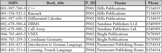
Fig. 6.1 Instance of relation BOOK_PUBLISHER

In this relation, there is repetition of names and phone numbers of publishers with all the books they have published. Now, assume that 100 books are published by any one publisher, and then all the information related to that publisher will be repeated unnecessarily over 100 tuples. In addition, due to redundancy, certain update anomalies can arise, which are as follows:

• Insertion anomaly: It leads to a situation in which certain information cannot be inserted in a relation unless some other information is stored. For example, in BOOK_PUBLISHER relation, information of a new publisher cannot be inserted unless he has not published any book. Similarly, information of a new book cannot be inserted unless information regarding publisher is not known.
• Deletion anomaly: It leads to a situation in which deletion of data representing certain information results in losing data representing some other information that is associated with it. For example, if the tuple with a given ISBN, say, 003-456-433-6 is deleted, the only information about the publisher P004 associated with that ISBN is also lost.
• Modification anomaly: It leads to a situation in which repeated data changed at one place results in inconsistency unless the same data is also changed at other places. For example, change in the name of a publisher, say, Hills Publications to Hills Publishers Pvt. Ltd. needs modification in multiple tuples. If the name of a publisher is not modified at all places, same P_ID will show two different values for publisher name in different tuples.

NOTE Modification anomaly cannot occur in case of a single relation as a single SQL query updates the entire relation. However, it can be a serious problem, if the data is repeated in multiple relations.

Fewer Null Values in Tuples

Sometimes, there may be a possibility that some attributes do not apply to all tuples in a relation. That is, values of all the attributes of a tuple are not known (as discussed in insertion anomaly). In that case, null value can be stored in those tuples. For example, in relation BOOK_PUBLISHER, detail of a new book without having information regarding publisher can be inserted by placing null values in all the attributes of publisher. However, null values do not provide complete solution as they cannot be inserted in the primary key attributes and the attributes for which not null constraint is specified. For example, detail of a new publisher who has not published any book cannot be inserted, as null value cannot be inserted in the attribute ISBN since it is a primary key. Moreover, null values waste storage space and may lead to some other problems such as interpreting them, accounting for them while applying aggregate functions such as COUNT or AVG, etc.

In a good database, the attributes whose values may frequently be null are avoided. If null values are unavoidable, they are applied in exceptional cases only. Thus, all the problems related to null values are minimized in a good database.

6.2 DECOMPOSITION

While designing a relational database schema, the problems that are confronted due to redundancy and null values can be resolved by decomposition. In decomposition, a relation is replaced with a collection of smaller relations with specific relationship between them. Formally, the decomposition of a relation schema R is defined as its replacement by a set of relation schemas such that each relation schema contains a subset of the attributes of R.

For example, the relation schema BOOK_PUBLISHER represents a bad design as it permits redundancy and null values, hence, it is undesirable. Thus, the schema of this relation requires to be modified so that it has less redundancy of information and fewer null values. The undesirable features from the relation schema BOOK_PUBLISHER can be eliminated by decomposing it into two relation schemas as given here.

BOOK_DETAIL(ISBN, Book_title, P_ID) and

PUBLISHER_DETAIL(P_ID, Pname, Phone)

The instances corresponding to the relation schemas BOOK_DETAIL and PUBLISHER_DETAIL are shown in Figure 6.2.

Fig. 6.2 Decomposition

From Figure 6.2, it is apparent that decomposition is actually a process of projection on a relation. Here, both the relations BOOK_DETAIL and PUBLISHER_DETAIL are the projections of original relation BOOK_PUBLISHER.

Now, a tuple for a new publisher can be inserted easily in relation PUBLISHER_DETAIL, even if no book is associated with that particular P_ID in relation BOOK_DETAIL. Similarly, a tuple for a particular P_ID in relation PUBLISHER_DETAIL can be deleted without losing any information (taking foreign key constraint into account). Moreover, name or phone for a particular P_ID can be changed by updating a single tuple in relation PUBLISHER_DETAIL. This is more efficient than updating several tuples and the scope for inconsistency is also eliminated.

During decomposition, it must be ensured that each attribute in R must appear in at least one relation schema Ri so that no attributes are lost. Formally,

 

∪ Ri = R

This is called attribute preservation property of decomposition.

NOTE There are two additional properties of decomposition, namely, lossless-join and dependency preservation property which are discussed in Section 6.5.

For smaller applications, it may be feasible for a database designer to decompose a relation schema directly. However, in case of large real-world databases that are usually highly complex, such a direct decomposition process is difficult as there can be different ways in which a relational schema can be decomposed. Further, in some cases, decomposition may not be required. Thus, in order to determine whether a relation schema should be decomposed and which relation schema may be better than another, some guidelines or formal methodology is needed. To provide such guidelines, several normal forms have been defined. These normal forms are based on the notion of functional dependencies that are one of the most important concepts in relational schema design.

6.3 FUNCTIONAL DEPENDENCIES

Functional dependencies are the special forms of integrity constraints that generalize the concept of keys. A given set of functional dependencies is used in designing a relational database in which most of the undesirable properties are not present. Thus, functional dependencies play a key role in developing a good database schema.

Definition: Let X and Y be the arbitrary subsets of set of attributes of a relation schema R, then an instance r of R satisfies functional dependency (FD) X → Y, if and only if for any two tuples t1 and t2 in r that have t1[X] = t2[X], they must also have t1[Y] = t2[Y]. That means, whenever two tuples of r agree on their X value, they must also agree on their Y value. Less formally, Y is functionally dependent on X, if and only if each X value in r is associated with it precisely one Y value.

The statement X → Y is read as Y is functionally dependent on X or X determines Y. The left and right sides of a functional dependency are called determinant and dependent, respectively.

Consider the relation schema BOOK_REVIEW_DETAIL(ISBN, Price, Page_count, R_ID, City, Rating) that represents review details of the books by the reviewers. The primary key of this relation is the combination of ISBN and R_ID. Note that the same book can be reviewed by different reviewers and same reviewer can review different books. The instance of this relation schema is shown in Figure 6.3.

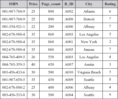
Fig. 6.3 An instance of BOOK_REVIEW_DETAIL relation

In this relation, the attribute Price is functionally dependent on the attribute ISBN (ISBN → Price), as tuples having same value for the ISBN have the same value for the Price. For example, the tuples having ISBN 001-987-760-9 have the same value 25 for Price. Similarly, the tuples having ISBN 002-678-980-4 have the same value 35 for Price. Other FDs such as ISBN → Page_count, Page_count → Price, R_ID → City are also satisfied. In addition, one more functional dependency {ISBN,R_ID} → Rating is also satisfied. That is, the attribute Rating is functionally dependent on composite attribute {ISBN,R_ID}.

While designing database, we are mainly concerned with the functional dependencies that must hold on relation schema R. That is, the set of FDs which are satisfied by all the possible instances that a relation on relation schema R may have. For example, in relation BOOK_REVIEW_DETAIL, the functional dependency Page_count → Price is satisfied. However, in real-world, the price of two different books having same number of pages can be different. So, it may be possible that at some time in an instance of relation BOOK_REVIEW_DETAIL, FD Page_count → Price is not satisfied. For this reason, Page_count → Price cannot be included in the set of FDs that hold on BOOK_REVIEW_DETAIL schema. Thus, a particular relation at any point in time may satisfy some FD, but it is not necessary that FD always hold on that relation schema.

The FDs can be represented conveniently by using FD diagram. In FD diagram, the attributes are represented as rectangular box. The arrow out of attribute depicts that on this attribute, the attributes to which arrow points are functionally dependent. The FD diagram for relation schema BOOK_REVIEW_DETAIL is shown in Figure 6.4.

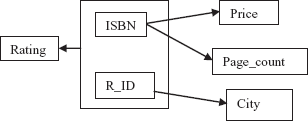
Fig. 6.4 FD diagram for BOOK_REVIEW_DETAIL

As stated earlier, while designing a database, the FDs that must hold on the relational schemas are specified. However, for a given relation schema, the complete set of FDs can be very large. For example, once again, consider the relation schema BOOK_REVIEW_DETAIL. In addition to the functional dependencies discussed earlier, some other FDs that hold on this relation schema are

        {R_ID, ISBN} → City
        {R_ID, ISBN} → {City, Rating}
        {R_ID, ISBN} → ISBN
        {R_ID, ISBN} → {R_ID, ISBN, City, Rating}

This large set of FDs can reduce the efficiency of database system. As each FD represents certain integrity constraint, the database system must ensure that any of the FDs should not be violated while performing any operation on the database. To reduce the effort spent in checking for violations, there should be some way to reduce the size of that set of FDs. That means for a particular set of FDs, say F₁, it is required to find some other set, say F₂, which is smaller than F₁ and every FD in F₁ is implied by FDs in F₂.

6.3.1 Trivial and Non-Trivial Dependencies

A dependency is said to be a trivial dependency if it is satisfied by all relations. For example, X → X is satisfied by all relations having attribute X. Similarly, XY → X is satisfied by all relations having attribute X. Generally, an FD A → B is trivial, if and only if B ⊆ A. Consider BOOK_REVIEW_DETAIL relation (see Figure 6.3). In this relation, the FDs like ISBN → ISBN and {R_ID, ISBN} → ISBN are trivial dependencies.

The dependencies, which are not trivial, are non-trivial dependencies. These are the dependencies that correspond to the essential integrity constraints. Thus, in practice, only non-trivial dependencies are considered. However, while dealing with the formal theory, all dependencies, trivial as well as non-trivial dependencies, have to be accounted.

6.3.2 Closure of a Set of Functional Dependencies

For a given set F of functional dependencies, some other dependencies also hold. That is, some functional dependencies are implied by F. For example, consider a relation schema R(A, B, C), such that both the FDs A → B and B → C hold for R. Then, FD A → C also holds on R as C is dependent on A transitively, via B. Thus, it can be said that FD A → C is implied.

The set of all FDs that are implied by a given set F of FDs is called the closure of F, denoted as F+. For a given F (if it is small), F⁺ can be computed directly. However, if F is large, then some rules or algorithms are needed to compute F⁺. Armstrong proposed a set of inference rules or axioms (also known as Armstrong’s axioms) to find logically implied functional dependencies. These rules are applied repeatedly for a given set F of functional dependencies, so that all of F⁺ can be inferred. Let A, B, C, and D be the arbitrary subsets of the set of attributes of a relation schema R and A ∪ B is denoted by AB, then these axioms can be stated as

• Reflexivity rule: If B ⊆ A, then A → B holds.
• Augmentation rule: If A → B holds, then AC → BC holds.
• Transitivity rule: If both A → B and B → C hold, then A → C holds.

The axioms are complete as for a given set F of FDs, all FDs implied by F can be inferred. The axioms are also sound as no additional FDs or incorrect FDs can be deduced from F using the rules. All the three axioms are proved for completeness and soundness. Though Armstrong’s axioms are complete and sound, computing F⁺ using them directly is a complicated task. Thus, to simplify the task of computing F⁺ from F, additional rules are derived from Armstrong’s axioms. These rules are as follows:

• Decomposition rule: If A → BC then A → B holds and A → C holds.
• Union rule: If A → B and A → C hold, then A → BC holds.
• Pseudotransitivity rule: If A → B holds and BC → D holds, then AC → D holds.

For example, consider a relation schema R(A, B, C, D, E, G) and the set F of functional dependencies { A → B, BC → D, D → E, D → G}. Some of the members of F⁺ of the given set F are

• AC → D. Since A → B and BC → D (Pseudotransitivity rule)
• BC → E. Since BC → D and D → E (Transitivity rule)
• D → EG. Since D → E and D → G (Union rule)

6.3.3 Closure of a Set of Attributes

In practice, there is little need to compute the closure of set of FDs. Generally, it is required to compute certain subset of the closure (subset consisting of all FDs with a specified set Z of attributes as determinant). However, to compute subset of closure, computing F⁺ is not an efficient process as F⁺ can be large. Moreover, computing F⁺ for a given set F of FDs involves applying Armstrong’s axioms repeatedly until they stop generating new FDs. So, some algorithm must be devised that can compute certain subset of the closure of the given set F of FDs without computing F⁺.

For a given relation schema R, a set Z of attributes of R and the set F of functional dependencies that hold on R, the set of all attributes of R that are functionally dependent on Z (known as the closure of Z under F, denoted by Z+) can be determined using the algorithm as shown in Figure 6.5.

  Z+ := Z;               //Initialize result to Z
  while(change in Z+) do // until change in result
   for each FD X → Y in F do //inner loop
   begin
       if X ⊆ Z+ //check if left hand side is subset
                 //of closure(result)
       then Z+ := Z+ U Y; //include the value on right hand
                         // side in result
   end

Fig. 6.5 Algorithm to Compute Z

For example, consider a relation schema R(A, B, C, D, E, G, H) and the set F of functional dependencies {A → B, BC → DE, AEG → H}. The steps to compute the closure {AC}⁺ of the set of attributes {A, C} under the set F of FDs (using algorithm given in Figure 6.5) are

1. Initialize the result Z⁺ to {A, C}.
2. On the execution of while loop first time, inner loop is repeated three times, once for each FD.
3. On the first iteration of the loop for A → B, since left hand side A is subset of Z⁺, include B in Z⁺. Thus, Z⁺ = {A, B, C}.
4. On the second iteration of the loop for BC → DE, include DE in Z⁺. Now Z⁺ = {A, B, C, D, E}.
5. On the third iteration of the loop for AEG → H, Z⁺ remains unchanged, since AEG is not subset of Z⁺.
6. On the execution of while loop second time, inner loop is repeated three times again. In all iterations, no new attribute is added in Z⁺, hence, the algorithm terminates. Thus, {AC}⁺ = {A, B, C, D, E}.

Besides, computing subset of closure, the closure algorithm has some other uses which are as follows.

• To determine if a particular FD, say X → Y is in the closure F⁺ of F, without computing the closure F+. This can be done by simply computing X⁺ by using closure algorithm and then checking if Y ⊆ X⁺.
• To test if a set of attributes A is a superkey of R. This can be done by computing A⁺, and checking if A⁺ contains all the attributes of R.

6.3.4 Equivalence of Sets of Functional Dependencies

Before discussing the equivalence sets of dependencies, one must be familiar with the term cover.

A set F2 of FDs is covered by another set F1 or F1 is cover of F2 if every FD in F2 can be inferred from F₁, that is, if every FD in F2 is also in F1⁺. This means, if any database system enforces FDs in F1, then FDs in F₂ will be enforced automatically.

Two sets F₁ and F₂ of FDs are said to be equivalent if F₁⁺ = F₂⁺, that is, every FD in F₁ is implied by F₂ and every FD in F₂ is implied by F₁. In other words, F₁ is equivalent to F₂, if both the conditions F1 covers F₂ and F₂ covers F₁ hold. It is clear from the definition, that if F₁ and F₂ are equivalent and the FDs in F₁ are enforced by any database system, then the FDs in F₂ will be enforced automatically and vice versa.

6.3.5 Canonical Cover

For every set of FDs, if a simplified set that is equivalent to given set of FDs can be generated, then the effort spent in checking the FDs can be reduced on each update. Since, simplified set will have the same closure as that of given set, any database that satisfies the simplified set of FDs will also satisfy the given set and vice versa. For example, consider a relation schema R(A, B, X, Y) with a set F of FDs AB → XY and A → Y. Now, whenever an update operation is applied on the relation, the database verifies both the FDs.

If we carefully examine the above given FDs, then we find that if we remove the attribute Y from the right-hand side of AB → XY, then it doesn’t affect the closure of F, since AB → X and A → Y implies AB → XY (by union rule). Thus, verifying AB → X and A → Y means same as that of verifying AB → XY and A → Y. However, verifying AB → X and A → Y requires less effort than checking the original set of FDs. This attribute X is extraneous in the dependency AB → XY, since the closure of new set is same as the closure of F. Formally, extraneous attribute can be defined as follows.

Consider a functional dependency X → Y in a given set F of FDs.

• Attribute A is extraneous in X if A ∈ X, and F logically implies (F–{X → Y}) ∪ {(X–A) → Y}.
• Attribute A is extraneous in Y if A ∈ Y, and the set of FDs (F–{X → Y}) ∪ {X → (Y–A)} logically implies F.

Once all such extraneous attributes are removed from the FDs, a new set say Fc is obtained. In addition, if the determinant of each FD in Fc is unique, that means, there are no two dependencies like X → Y and X → Z in Fc, then Fc is called canonical cover for F.

A canonical cover for a set of functional dependencies can be computed by using the algorithm given in Figure 6.6.

  Fc := F;
  while(change in Fc) do
    replace any FD in Fc of the form X → A, X → B
         with X → AB (Use union rule)
    for(each FD X → Y in Fc)do
    begin
      if(extraneous attribute is found either in X or in Y)
      then remove it from X → Y
    end

Fig. 6.6 Algorithm to compute canonical cover for F

To illustrate the algorithm given in Figure 6.6, consider a set F of functional dependencies {A → C, AC → D, E → AD, E → H} on relation schema R(A,B,C). To compute the canonical cover for a set F, follow these steps.

1. Initialize Fc to F.
2. On first iteration of the loop, replace FDs E → AD and E → H with E → ADH, as both these FDs have same set of attributes in determinant (left side of FD). Now, Fc = {A → C, AC → D, E → ADH}. In FD AC → D, C is extraneous. Thus, Fc = {A → C, A → D, E → ADH}.
3. On second iteration, replace FDs A → C and A → D with A → CD. Now, Fc = {A → CD, E → ADH}. In FD A → CD, no attribute is extraneous. In FD E → ADH, D is extraneous. Thus, Fc = {A → CD, E → AH}.
4. On third iteration, the loop terminates, since determinant of each FD is unique and no extraneous attribute is there. Thus, Fc (canonical cover) is {A → CD and E → AH}.

It is obvious that the canonical cover of F, Fc has same closure as F. This implies, if we have determined that Fc is satisfied, then we can say F is also satisfied. Moreover, Fc is minimal as FDs with same left side have been combined and Fc does not contain extraneous attributes. Thus, it is easier to test Fc than to test F itself.

6.4 NORMAL FORMS

Consider a relation R with a designated primary key and a set F of functional dependencies. To decide whether the relation is in desirable form or it should be decomposed into smaller relations, some guidelines or formal methodology is needed (as stated earlier). To provide such guidelines, several normal forms have been defined (see Figure 6.7).

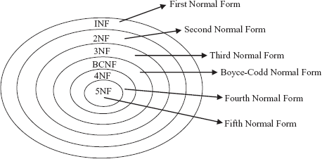
Fig. 6.7 Normal forms

A relation is said to be in a particular normal form if it satisfies certain specified constraints. Each of the normal forms is stricter than its predecessors. The normal forms are used to ensure that various types of anomalies and inconsistencies are removed from the database.

Initially, Codd proposed three normal forms namely, first normal form (1NF), second normal form (2NF), and third normal form (3NF). There were certain inadequacies in the third normal form, so a revised definition was given by Boyce and Codd. This new definition is known as Boyce-Codd normal form (BCNF) to distinguish it from the old definition of third normal form. This new definition is stricter than the old definition of third normal form as any relation which is in BCNF is also in third normal form; however, reverse may not be true. All these normal forms are based on the functional dependency. Two other normal forms, namely, fourth normal form (4NF) and fifth normal form (5NF) have been proposed which are based on the concepts of multivalued dependency and join dependency, respectively.

The process of modifying a relation schema so that it conforms to certain rules (normal forms) is called normalization. Normalization is conducted by evaluating a relation schema to check whether it satisfies particular rules and if not, then decomposing schema into set of smaller relation schemas that do not violate those rules. Normalization can be considered as fundamental to the modeling and design of a relational database, the main purpose of which is to eliminate data redundancy and avoid data update anomalies.

Generally, it is desirable to normalize the relation schema in a database to the highest possible form. However, normalizing a relation schema to higher forms can introduce complexity to the design and application. As it results in more relations and more relations need more join operations while carrying out queries in database system which can decrease the performance. Thus, while normalization, performance should be taken into account that may result in a decision not to normalize beyond third normal form or BCNF normal form.

NOTE Redundancy cannot be minimized to zero in any database system.

6.4.1 First Normal Form

The first normal form states that every tuple must contain exactly one value for each attribute from the domain of that attribute. That is, multivalued attributes, composite attributes, and their combinations are not allowed in 1NF.

Definition: A relation schema R is said to be in first normal form (1NF) if and only if the domains of all attributes of R contain atomic (or indivisible) values only.

Consider the relation schema BOOK_INFO{ISBN, Price, Page_count, P_ID, R_ID, rating} that represents the information regarding books and reviews. The functional dependencies that hold on relation schema BOOK_INFO are {ISBN → Price, Page_count, P_ID} and {ISBN, R_ID → Rating}. The only key of the relation BOOK_INFO is the combination of ISBN and R_ID. For the purpose of explaining normalization, an additional constraint Page_count → Price is introduced. It implies that price of book is determined by the number of pages in the book. The FD diagram for BOOK_INFO is shown in Figure 6.8 and corresponding instance is shown in Figure 6.9.

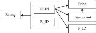
Fig. 6.8 FD diagram for BOOK_INFO

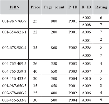
Fig. 6.9 Unnormalized relation BOOK_INFO

It is clear from Figure 6.9 that tuples contain multiple values for some of the attributes. For example, the tuple for ISBN 001-987-760-9 has two values for the attributes R_ID and Rating. Thus, it is an unnormalized relation. A relation is said to be an unnormalized relation if it contains non-atomic values. This relation can be normalized into 1NF by creating one tuple for each value in multivalued attributes as shown in Figure 6.10.

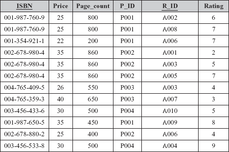
Fig. 6.10 Relation BOOK_INFO in 1NF

A good database design always requires that domains of all the attributes of a relation must be atomic, so that the relation schemas are in 1NF. However, depending on the requirement or from the performance point of view, sometimes non-atomic values are useful. For instance, a single attribute Address can be used to hold house number, street, city such as 12, Park street, Atlanta in a relation. Whether the house number, the street name, and city should be separated into distinct attributes depends on how data is to be used. For example, if the address for mailing is needed only, then a single attribute Address can be used. However, if the information like all the publishers in a given street is required, then house number, the street name, and city should constitute their own attributes.

NOTE Modern database system supports non-atomic values.

Though the BOOK_INFO is in 1NF, it has some shortcomings. The information regarding the same book is repeated a number of times. Further, there are certain anomalies with respect to update operations. For example, the information of a new book cannot be inserted unless some reviewer reviews it. In addition, the change in the price of a book for particular ISBN can lead to inconsistency in the database, if it is not changed in all the tuples where the same ISBN appears. Moreover, the deletion of information of rating for a book having ISBN, say, 003-456-533-8 can cause the loss of detail of the book. This is because there exists only one tuple that contains this particular ISBN. Thus, to resolve these problems, this schema needs further normalization.

6.4.2 Second Normal Form (2NF)

The second normal form is based on the concept of full functional dependency. An attribute Y of a relation schema R is said to be fully functional dependent on attribute X (X → Y), if there is no A, where A is proper subset of X such that A → Y. It implies removal of any attribute from X means that the dependency does not hold any more. A dependency X → Y is a partial dependency if there is any attribute A where A is proper subset of X such that A → Y.

For example, consider the relation schema BOOK_INFO in which the attributes ISBN and R_ID together form the key. In this schema, the attribute Rating is fully functional dependent on the key {ISBN, R_ID} as Rating is not dependent on any subset of key. That is, neither ISBN → Rating nor R_ID → Rating holds. However, the attributes Price, Page_count, P_ID are partially dependent on key, since they are dependent on ISBN, which is a subset of key {ISBN, R_ID}.

Definition: A relation schema R is said to be in second normal form (2NF) if every non-key attribute A in R is fully functionally dependent on the primary key. An attribute is non-key or non-prime attribute, if it is not a part of candidate key of R.

Consider once again, the relation schema BOOK_INFO. This schema is not in 2NF as it involves partial dependencies. This schema can be normalized to 2NF by eliminating all partial dependency between a non-key attribute and the key. This can be achieved by decomposing BOOK_INFO into two relation schemas as follows:

  BOOK{ISBN,Price, Page_count, P_ID}
  REVIEW {ISBN,R_ID, Rating}

The instances corresponding to the relation schemas BOOK and REVIEW are shown in Figure 6.11.

Fig. 6.11 Relations in 2NF

The relation schemas BOOK and REVIEW do not have any partial dependencies. Each of the nonkey attributes of relation schemas BOOK and REVIEW is fully functional dependent on key attribute ISBN and (ISBN, R_ID), respectively. Hence, both the schemas are in 2NF. The FDs corresponding to these relation schemas are shown in Figure 6.12.

Fig. 6.12 FDs in 2NF

Now, all the problems of BOOK_INFO have been overcome by normalizing it into 2NF; however, the decomposed relation schema BOOK which is in 2NF still causes problems over update operation. For example, the Price for Page_count 900 cannot be inserted unless there exists a book having 900 pages. Similarly, the change in the Price for particular Page_count can lead to inconsistency in the database if all the tuples where the same Page_count appears are not changed. Moreover, the deletion of the Price for particular Page_count say, 200 can cause the loss of information of the book having ISBN 001-354-921-1. This is due to the fact that there exists only one tuple that contains the information of book having this particular ISBN. These problems can be resolved by normalizing this relation schema further. Since, relation schema REVIEW do not have such type of anomalies, there is no need to normalize it further.

6.4.3 Third Normal Form (3NF)

The third normal form is based on the concept of transitive dependency. An attribute Y of a relation schema R is said to be transitively dependent on attribute X (X → Y), if there is set of attributes A that is neither a candidate key nor a subset of any key of R and both X → A and A → Y hold. For example, the dependency ISBN → Price is transitive through Page_count in relation schema BOOK. This is because both the dependencies ISBN → Page_count and Page_count → Price hold and Page_count is neither a candidate key nor a subset of candidate key of BOOK.

Definition: A relation schema R is in third normal form (3NF) with a set F of functional dependencies if, for every FD X → Y in F, where X be any subset of attributes of R and Y be any single attribute of R, at least one of the following statements hold

• X → Y is a trivial FD, that is, Y ⊆ X.
• X is a superkey for R.
• Y is contained in a candidate key for R.

It can also be stated as,

A relation schema R is in third normal form (3NF) if and only if it satisfies 2NF and every nonkey attribute is non-transitively dependent on the primary key.

For example, the schema BOOK can be decomposed into two relation schemas say, BOOK_PAGE and PAGE_PRICE to eliminate transitive dependency between the attributes ISBN and Price. Hence, the schemas BOOK_PAGE and PAGE_PRICE are in 3NF. The instances of these schemas are shown in Figure 6.13, and Figure 6.14 shows FD diagrams of these schemas.

Note that this definition of 3NF can be used to handle relations in which primary key is the only candidate key. Thus, to handle the relations having more than one candidate key, this old definition of 3NF was replaced by new definition by Boyce and Codd normal form which is also known as BCNF.

Fig. 6.13 Relations in 3NF

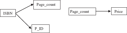
Fig. 6.14 FD diagram for BOOK_PAGE and PAGE_PRICE

6.4.4 Boyce-Codd Normal Form (BCNF)

Boyce-Codd normal form was proposed to deal with the relations having two or more candidate keys that are composite and overlap. Two candidate keys overlap if they contain two or more attributes and have at least one attribute in common.

Definition: A relation schema R is in Boyce-Codd normal form (BCNF) if, for every FD X → A in F, where X is the subset of the attributes of R, and A is an attribute of R, one of the following statements holds

• X → Y is a trivial FD, that is, Y ⊆ X.
• X is a superkey.

In simple terms, it can be stated as

A relation schema R is in BCNF if and only if every non-trivial FD has a candidate key as its determinant.

For example, consider a relation schema BOOK(ISBN, Book_title, Price, Page_count) with two candidate keys, ISBN and Book_title. Further, assume that the functional dependency Page_count → Price no longer holds. The FD diagram for this relation schema is shown in Figure 6.15.

As shown in Figure 6.15, there are two determinants ISBN and Book_title and both of them are candidate keys. Thus, this relation schema is in BCNF.

BCNF is the simpler form of 3NF as it makes explicit reference to neither the first and second normal forms, nor to the concept of transitive dependence. Furthermore, it is stricter than 3NF as every relation which is in BCNF is also in 3NF, but vice versa is not necessarily true. A 3NF relation will not be in BCNF if there are multiple candidate keys in the relation such that

• the candidate keys in the relation are composite keys, and
• the keys are not disjoint, that is, candidate keys overlap.

To illustrate this point, consider a relation schema BOOK_RATING(ISBN, Book_title, R_ID, Rating). The candidate keys are (ISBN, R_ID) and (Book_title, R_ID). This relation schema is not in BCNF since both the candidate keys are composite as well as overlapping. However, it is in 3NF.

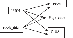
Fig. 6.15 FD diagrams for BOOK and with Book_title as candidate key

Fig. 6.16 Instance of relation BOOK_RATING

From the instance corresponding to this relation schema as shown in Figure 6.16, it is clear that it suffers from the problem of repetition of information. Thus, changing the title of book can cause logical inconsistency if it is not changed in all the tuples in which it appears. This problem can be resolved by decomposing this relation schema into two relation schemas as shown here.

  BOOK_TITLE_INFO(ISBN, Book_title) and
  REVIEW(R_ID, ISBN, Rating)

Or

  BOOK_TITLE_INFO(ISBN, Book_title) and
  REVIEW(R_ID, Book_title, Rating)

Now, all these relation schemas are in BCNF. Note that BCNF is the most desirable normal form as it ensures the elimination of all redundancy that can be detected using functional dependencies.

 

6.5 INSUFFICIENCY OF NORMAL FORMS

From the discussion so far, it can be concluded that generally normalization start from a single universal relation which includes all attributes of a database. The relation is decomposed repeatedly until a BCNF or 3NF is achieved. However, this condition is not sufficient on its own to guarantee a good relational database schema design. In addition to this condition, there are two additional properties that must hold on decomposition to qualify it as a good design. These are lossless-join property and dependency preservation property.

6.5.1 Lossless-Join Property

The notion of the lossless-join property is crucial as it ensures that the original relation must be recovered from the smaller relations that result after decomposition. That is, it ascertains that no information is lost after decomposition.

Definition: Let R be a relation schema with a given set F of functional dependencies. Then decomposition D = {R1, R2, …, Rn} on R is said to be lossless (lossless–join), if for every legal relation (that is, relation that satisfies the specified functional dependencies and other constraints), following statement holds.

ΠR1 (R) ΠR2 (R) … ΠRn (R)= R

In other words, if the original relation can be reconstructed by combining the projections of a relation using natural join (or the process of decomposition is reversible), decomposition is lossless decomposition, otherwise, it is a lossy (lossy–join) decomposition.

For example, consider again the relation schema BOOK(ISBN, Price, Page_count) with the functional dependencies ISBN → Price and Page_count → Price. Other attributes are ignored to simplify the relation schema. An instance of this relation schema is shown in Figure 6.17.

The relation schema BOOK(ISBN, Price, Page_count) can be decomposed in two different ways, say, decomposition A and decomposition B (see Figure 6.17). The schemas corresponding to decomposition A and decomposition B are given here.

Decomposition A

BOOK_PRICE(ISBN, Price)

and BOOK_PAGES(ISBN, Page_count)

Decomposition B

BOOK_PRICE(ISBN, Price)

and PRICE_PAGE(Price, Page_count)

Fig. 6.17 Instance of relation BOOK and two corresponding decompositions

In Decomposition A (see Figure 6.17), the price and the number of pages for all the books can be determined easily. Since, no information is lost in this decomposition, decomposition A is lossless.

In Decomposition B (see Figure 6.17), it can be determined that price of the books having ISBN 001-987-760-9 and 002-678-980-4 is 25. However, the number of pages in these books cannot be determined as there are two values for page_count in relation PRICE_PAGE corresponding to the Price 25. Thus, this decomposition is lossy.

If an decomposition does not have the lossless-join property, then additional spurious tuples (tuples that are not in original relation) may be obtained on applying join operation on the relations resulted after decomposition. These spurious tuples represent erroneous data. For example, consider the relations BOOK_PRICE and PRICE_PAGE as shown in decomposition B in Figure 6.17. If these relations are joined, a new relation having additional spurious tuples is obtained as shown in Figure 6.18.

Fig. 6.18 Relation with spurious tuples

However, if the relations as shown in decomposition A in Figure 6.17 are joined, no spurious tuples will be generated. Thus, if lossless-join property holds on decomposition, it is ensured that no spurious tuples are obtained when a natural join operation is applied to the relations resulted after decomposition. So, this property is also known as non-additive join property.

A particular decomposition can be tested for having lossless property on the basis of functional dependency by applying the property as given here.

Lossless-join test for binary decompositions: Let R be a relation schema with F a set of FDs over R. The decomposition of R into two relations R1 and R2 form a lossless decomposition if at least one of the following dependencies is in F⁺.

  R1 ∩ R2 → R1 – R2
  R1 ∩ R2 → R1 – R2

This property is limited to binary decompositions (decomposition of a relation into two relations) only. In addition, it is a necessary condition only if all constraints are functional dependencies.

NOTE The test for lossless decomposition in case of a decomposition of a relation into multiple relations is beyond this discussion.

6.5.2 Dependency Preservation Property

Another important property that is desired while decomposition is dependency preservation, that is, no FD of the original relation is lost. Consider a relation schema R with set F of FDs {X → Y, Y → Z}. One other dependency that is implied from F is X→ Z. Let R is decomposed into two relation schemas, R1{X,Y} with FD X → Y and R2{Y,Z} with FD Y → Z. Here, X → Z is enforced automatically since it is implied from FDs of R1 and R2. Hence, this decomposition is dependency preserving. Now, suppose that R is decomposed into two relation schemas, R1{X,Y} with FD X → Y and R2{X,Z} with FD X → Z. Here, FD Y → Z is not implied from R1 and R2. To enforce this FD, join operation is to be applied whenever a new tuple is to be inserted. We know that computing join is a costly process in terms of CPU usage and response time.

Dependency preservation property ensures that each FD represented by original relation is enforced by examining any single relation resulted from decomposition or can be inferred from the FDs in some decomposed relation. Thus, it prevents computation of join. To understand this property, let us first understand the term projection. Given a relation schema R with set F of FDs and R1, R2,…, Rn be the decomposition of R, the projection of F to Ri is the set Fi of all FDs in F⁺ (not just F) that include only attributes of Ri. For example, once again consider the decomposition of R1{X,Y} and R2{X,Z} of R. The projection of F to R1, denoted by FR1 is X → Z, since X → Z in F⁺, even though it is not in F. This FD can be tested by examining relation R2 only. Similarly, FDs in each projection can be tested by analyzing only one relation in the decomposed set.

However, testing each projection is not sufficient to determine whether the decomposition is dependency preserving. Since, it is not always necessary that all the dependencies in original relation appear directly in an individual decomposed relation. That is, there may be FDs in F⁺ that are not the projections. Thus, we also need to examine the FDs that are inferred from the projections. Formally, the decomposition of relation schema R with a given set F of FDs into relations R1, R2, …, Rn is dependency preserving if F’⁺ = F⁺, where F’= FR1 ∪ FR2∪… ∪ FRn.

 

6.6 COMPARISON OF BCNF AND 3NF

From the discussion so far, it can be concluded that the goal of a database design with functional dependencies is to obtain schemas that are in BCNF, are lossless and preserves the original set of FDs.

A relation can always be decomposed into 3NF in such a way that the decomposition is lossless and dependency preserving. However, there are some disadvantages to 3NF. There is a possibility that null values are used to represent some of the meaningful relationships among data items. In addition, there is always a scope of repetition of information.

On the other hand, it is always not possible to obtain a BCNF design without sacrificing dependency preservation. For example, consider a relation schema CITY_ZIP(City, Street, Zip) with FDs {City, Street} → Zip and Zip → City is decomposed into two relation schemas R1(Street, Zip) and R2(City, Zip). It is observed that both these schemas are in BCNF. In R1, there is only trivial dependency and in R2, the dependency Zip → City holds. It can be seen clearly that the FD {City, Street} → Zip is not implied from decomposed relation schemas. Thus, this decomposition does not preserve dependency, that is, (F1 ∪ F2)+ ≠ F⁺_, where F1 and F2 are the restrictions of R1 and R2, respectively.

Clearly, it is not always possible to achieve the goal of database design. In that case, we have to be satisfied with relation schemas in 3NF rather than BCNF. This is because, if dependency preservation is not checked efficiently, either system performance can be reduced or it may risk the integrity of the data. Thus, maintaining the integrity of data at the cost of the limited amount of redundant data is a better option.

6.7 HIGHER NORMAL FORMS

As stated earlier, BCNF is the desirable normal form; however, some relation schemas even though they are in BCNF still suffer from the problem of repetition of information. For example, consider an alternative design for Online Book database having a relation schema BOOK_AUTHOR_DETAIL(ISBN, A_ID, Phone). An instance of this relation schema is shown in Figure 6.19(a).

In this relation, there are two multivalued attributes, A_ID and Phone that represents the fact that a book can be written by multiple authors and an author can have multiple phone numbers. That is, for a given ISBN, there can be multiple values in attribute A_ID and for a given A_ID, there can be multiple values for attribute Phone. To make the relation consistent, every value of one of the attributes is to be repeated with every value of the other attribute [see Figure 6.19(b)].

Fig. 6.19 Relation BOOK_AUTHOR_DETAIL

From Figure 6.19(b), it is clear that relation BOOK_AUTHOR_DETAIL satisfies only trivial dependencies. In addition, it is all key relation (a relation in which key is the combination of all the attributes taken together) and any all key relation must necessarily be in BCNF. Thus, this relation is in BCNF. However, it involves lot of redundancies which leads to certain update anomalies. Thus, it is always not possible to decompose a relation on the basis of functional dependencies to avoid redundancy.

NOTE BCNF can eliminate the redundancies that are based on the functional dependencies.

 

Since, normal forms based on functional dependencies are not sufficient to deal such type of situations, other type of dependencies and normal forms have been defined.

6.7.1 Multivalued Dependencies

Multivalued dependencies (MVDs) are the generalization of functional dependencies. Functional dependencies prevent the existence of certain tuples in a relation. For example, if a FD X → Y holds in R, then any r(R) cannot have two tuples having same X value but different Y values. On the contrary, multivalued dependencies do not rule out the presence of those tuples, rather, they require presence of other tuples of a certain form in the relation. Multivalued dependencies arise when a relation having a non-atomic attribute is converted to a normalized form. For each X value in such a relation, there exists a well-defined set of Y values associated with it. This association between the X and Y values does not depend on the values of the other attributes in the relation.

To understand the notion of multivalued dependencies more clearly, consider the relation BOOK_AUTHOR_DETAIL as shown in Figure 6.19(a). In this relation, although the ISBN does not have a unique A_ID (the FD ISBN → A_ID does not hold), each ISBN has a well defined set of corresponding A_ID. Similarly for a particular A_ID, a well defined set of Phone exists. In addition, book is independent of the phone numbers of authors, due to which there is lot of redundancy in this relation. Such situation which cannot be expressed in terms of FD is dealt by specifying a new form of constraint called multivalued dependency or MVD.

Definition: In a relation schema R, an attribute Y is said to be multi-dependent on attribute X (X →→ Y) if and only if for a particular value of X, the set of values of Y is completely determined by the value of X alone and is independent of the values of Z where, X, Y, and Z are the subsets of the attributes of R.

X →→ Y is read as Y is multi-dependent on X or X multi-determines Y.

From the definition of MVD, it is clear that if X → Y, then X →→ Y. In other words, every functional dependency is a multivalued dependency. However, the converse is not true.

The multivalued dependencies that hold in the relation BOOK_AUTHOR_DETAIL, [see Figure 6.19(b)] can be represented as

  ISBN →→ A_ID
  A_ID →→ Phone

If the MVD X →→ Y is satisfied by all relations on schema R, then X →→ Y is a trivial dependency on schema R, that is, X →→ Y is trivial if Y ⊆ X or Y ∪ X = R.

NOTE Generally, the relations containing non-trivial MVDs are all key relations.

 

Like functional dependencies (FDs), inference rules for multivalued dependencies (MVDs) have been formulated which are complete as well as sound. These set of rules consist of three Armstrong axioms (discussed earlier) and five additional rules. Three of these rules involve only MVDs which are

• Complementation rule for MVDs: If X →→ Y, then X →→ R–XY.
• Augmentation rule for MVDs: If X →→ Y and W ⊇ Z, then WX →→ YZ.
• Transitive rule for MVDs: If X →→ Y and Y →→ Z, then X →→ (Z–Y).

The remaining two inference rules relate FDs and MVDs. These rules are

• Replication rule for FD to MVD: If X → Y, then X →→ Y.
• Coalescence rule for FD to MVD: If X →→ Y and there exists W such that W ∩ Y is empty, W → Z and Y ⊇ Z, then X → Z.

6.7.2 Fourth Normal Form

Fourth normal form is based on the concept of multivalued dependency. It is required when undesirable multivalued dependencies occur in a relation. This normal form is more restrictive than BCNF. That is, any 4NF is necessarily in BCNF but converse is not true.

Definition: A relation schema R is in fourth normal form (4NF) with respect to a set F of functional and multivalued dependencies if, for every non-trivial multivalued dependency X →→ Y in F+, where X ⊆ R and Y ⊆ R, X is a superkey of R.

For example, consider, once again relation BOOK_AUTHOR_DETAIL. As stated earlier, the problem is due to the fact that book is independent of the phone number of authors. This problem can be resolved by eliminating this undesirable dependency, that is, by decomposing this relation into two relations BOOK_AUTHOR and AUTHOR_PHONE as shown in Figure 6.20.

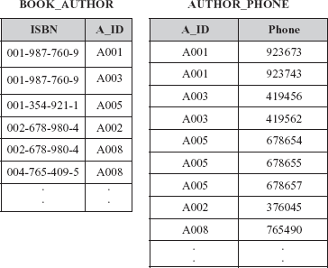
Fig. 6.20 Relations in 4NF

Since, the relations BOOK_AUTHOR and AUTHOR_PHONE do not involve any MVD, they are in 4NF. Hence, this design is an improvement over the original design. Further, relation BOOK_AUTHOR_DETAIL can be recovered by joining BOOK_AUTHOR and AUTHOR_PHONE together.

Note that whenever a relation schema R is decomposed into relation schemas R₁ = (X ∪ Y) and R2 = (R–Y) based on MVD X →→ Y that holds in R, the decomposition has the lossless-join property. This condition is necessary and sufficient for decomposing a schema into two schemas that have lossless-join property. Formally, this condition can be stated as:

Property for lossless-join decomposition into 4NF: The relation schemas R₁ and R₂ form lossless-join decomposition of R with respect to a set F of functional and multivalued dependencies if and only if

  (R1 ∩ R2) →→ (R1 - R2) or
  (R1 ∩ R2) →→ (R1 - R2)

6.7.3 Join Dependencies

The property (lossless-join test for binary decompositions) that is discussed earlier, gives the condition for a relation schema to be decomposed in a lossless way by exactly two of its projections. However, in some cases, there exist relations that cannot be lossless decomposed into two projections but can be lossless decomposed into more than two projections. Moreover, it may be in 4NF that means there may neither any functional dependency in R that violates any normal form upto BCNF nor any non-trivial dependency that violates 4NF. However, the relation may have another type of dependency called join dependency which is the most general form of dependency possible.

Consider a relation AUTHOR_BOOK_PUBLISHER (see Figure 6.21) which is all key relation (all the attributes form key). Since, in this relation, no non-trivial FDs or MVDs are involved, it is in 4NF. It should be noted that if it is decomposed exactly into any two relations and joined back, a spurious tuple is created (see Figure 6.21); however, if it is decomposed into three relations and joined back as shown in Figure 6.21, original relation is obtained. It is because it specifies another constraint according to which, whenever an author a writes book b, and a publisher p publishes book b, and the author a writes at least one book for publisher p, then author a will also be writing book b for publisher p. For example,

If a tuple having values <A001, C++> exists in AUTHOR_BOOK

and a tuple having values <C++, P001> exists in BOOK_PUBLISHER

and a tuple having values <P001, A001> exists in PUBLISHER_AUTHOR

then a tuple having values <A001, C++, P001> exists in AUTHOR_BOOK_PUBLISHER

Note that the converse of this statement is true, that is, if <A001, C++, P001> appears in AUTHOR_BOOK_PUBLISHER, then <A001, C++> appears in relation AUTHOR_BOOK and so on. Further, <A001, C++> appears in AUTHOR_BOOK if and only if <A001, C++, P002> appears in AUTHOR_BOOK_PUBLISHER for some P002 and similarly, for <C++, P001> and <P001, A001>. This statement can be rewritten as a constraint on AUTHOR_BOOK_PUBLISHER as “If tuples having values <A001, C++, p002> <A002, C++, P001> and <A001, Unix, P001 > exists in AUTHOR_BOOK_PUBLISHER then tuple having values <A001, C++, P001> also exists in AUTHOR_BOOK_PUBLISHER”.

Since, this constraint is satisfied if and only the relation is joining of certain projections, this constraint is referred as join dependency (JD).

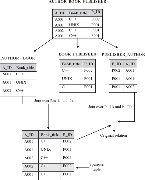
Fig. 6.21 Non-loss decomposition of a relation into three projections

Definition: Let R be a relation schema and R₁, R₂, …, R_n be the decomposition of R, R is said to satisfy the join dependency *(R₁, R₂, …, R_n) (read as “star R₁, R₂, …, R_n”), if and only if

 

ΠR1 (R) ΠR2 (R) … ΠRn (R) = R

In other words, relation schema R satisfies the JD *(R₁, R₂, …, R_n) if and only if every legal instance r(R) is equal to join of its projections on R₁, R₂, …, R_n.

From this definition, it is clear that MVD is a special case of a JD, where n = 2 (or join dependency is generalization of MVD). A join dependency *(R₁, R₂, …, R_n) specified on a relation schema R is a trivial JD, if at least one relation schema R_i in JD *(R₁, R₂, …, R_n) is the set of all attributes of R (that is, one of the relation schemas R_i in JD *(R₁, R₂, …, R_n) is equal to R). Such a dependency is called trivial because it has the lossless-join property for any instance of R and hence, does not specify any constraint on R.

6.7.4 Fifth Normal Form

Fifth Normal Form also called project–join normal form (PJ/NF) is based on the concept of join dependencies.

Definition: A relation schema R is in fifth normal form (5NF) with respect to a set F of functional, multivalued, and join dependencies if, for every non-trivial join dependency *(R₁, R₂, …, R_n) in F+, every R_i is a superkey of R.

For example, consider once again the AUTHOR_BOOK_PUBLISHER relation (see Figure 6.21) which satisfies join dependency that is not implied by its sole superkey (that key being the combination of all its attributes). Thus, it is not in 5NF. In addition, this relation suffers from a number of update anomalies. These anomalies can be eliminated if it is decomposed into three relations AUTHOR_BOOK, BOOK_PUBLISHER, and PUBLISHER_AUTHOR. Each of these relations is in 5NF since they do not involve any join dependency. Further, if join operation is applied on any two of these relations, spurious tuples are generated; however, it is not so on applying join operation on all three relations. Note that any relation in 5NF is automatically in 4NF.

6.8 DENORMALIZATION

From the discussion so far, it is clear that when the process of normalization is applied to a relation, the redundancy is reduced. However, it results in more relations which increase the CPU overhead. Hence, it fails to provide adequate response time, that is, makes the database system slow which often counteracts the redundant data. Thus, sometimes, in order to speed up database access, the relations are required to be taken from higher normal form to lower normal form. This process of taking a schema from higher normal form to lower normal form is known as denormalization. It is mainly used to improve system performance to support time-critical operations. There are several other factors which require denormalizing relations are given here.

• Many critical queries that require data to be retrieved from more than one relation.
• Many computations need to be applied to one or many attributes before answering a query.
• The values in multivalued attributes need to be processed in a group instead of individually.
• Relations need to be accessed in different ways by different users during same duration.

Like normalization, there is no formal guidance that outlines the approach to denormalizing a database. Once the process of denormalization is started, it is not clear where should it be stopped. Further, the relations that are denormalized suffer from a number of other problems like redundancy and update problems. It is obvious as the relations, which are to be dealt are once again the relations that are less than fully normalized. Moreover, denormalization makes certain queries harder to express. Thus, the main aim of denormalization process is to balance the need for good system response time and need to maintain data while avoiding the various problems associated with denormalized relations.

1. Designing of relation schemas is based on the conceptual design. The relation schemas can be generated directly using conceptual data model such as ER or enhanced ER (EER) or some other conceptual data model. The goodness of the resulting set of schemas depends on the designing of the data model.
2. A relational database is considered as good if it has minimum redundancy and null values.
3. While designing relational database schema, the problems that are confronted due to redundancy and null values can be resolved by decomposition.
4. In decomposition, a relation is replaced with a collection of smaller relations with specific relationship between them.
5. During decomposition, it must be ensured that each attribute in R must appear in at least one relation schema Ri so that no attributes are lost. This is called attribute preservation property of decomposition.
6. Functional dependencies are one of the most important concepts in relational schema design. They are the special forms of integrity constraints that generalize the concept of keys. A given set of functional dependencies is used in designing a relational database in which most of the undesirable properties are not present.
7. For a given set F of functional dependencies, some other dependencies also hold. That is, some functional dependencies are logically implied by F. The set of all FDs that are implied by a given set of FDs is called the closure of F, denoted as F+.
8. Armstrong proposed a set of inference rules or axioms (also known as Armstrong’s axioms) to find logically implied functional dependencies. The axioms are complete and sound.
9. Two sets F1 and F2 of FDs are said to be equivalent if F1+ = F2+, that is, every FD in F1 is implied by F2 and every FD in F2 is implied by F1.
10. For every set of FDs, canonical cover (a simplified set) that is equivalent to given set of FDs can be generated.
11. To determine the quality or goodness of a database, some formal measures or guidelines are required. Normalization theory provides the guidelines to assess the quality of a database in designing process. The normalization is the application of set of simple rules called normal forms to the relation schema.
12. A relation is said to be in a particular normal form if it satisfies certain specified constraints.
13. A relation is said to be an unnormalized relation if it contains non-atomic values.
14. Four normal forms, namely, first normal form (1NF), second normal form (2NF), third normal form (3NF), and Boyce-Codd normal form (BCNF) are based on the functional dependency.
15. A relation is said to be in first normal form (1NF) if the domains of all its attributes contain atomic (or indivisible) values only.
16. The second normal form is based on the concept of full functional dependency.
17. The third normal form is based on the concept of transitive dependency.
18. Boyce-Codd normal form was proposed to deal with the relations having two or more candidate keys that are composite and overlap.
19. There are two additional properties that must hold on decomposition to qualify a relational schema as a good design. These are lossless-join property and dependency preservation property.
20. Lossless-join property ensures that the original relation must be recovered from the smaller relations that result after decomposition.
21. Dependency preservation property ensures that each FD represented by original relation is enforced by examining any single relation resulted from decomposition or can be inferred from the FDs in some decomposed relation.
22. Lossless-join property is indispensable requirement of decomposition that must be achieved at any cost, whereas the dependency preservation property, though desirable, can be sacrificed sometimes.
23. Normal forms based on functional dependencies are always not sufficient to avoid redundancy. So, other types of dependencies and normal forms have been defined.
24. Multivalued dependencies (MVDs) are the generalization of functional dependencies.
25. Fourth normal form is based on the concept of multivalued dependency. It is required when undesirable multivalued dependencies occur in a relation.
26. A relation may have another type of dependency called join dependency which is the most general form of dependency possible.
27. Fifth normal form (5NF), also called project–join normal form (PJ/NF) is based on the concept of join dependencies.
28. The process of normalization is applied to a relation to reduce redundancy. However, it results in more relations which increase the CPU overhead.
29. In order to speed up database access, the relations are required to be taken from higher normal form to lower normal form. This process of taking a schema from higher normal form to lower normal form is known as denormalization.

• Decomposition
• Attribute preservation property
• Functional dependency
• Determinant and dependent
• Trivial dependency
• Non-trivial dependencies
• Closure of a set of functional dependencies
• Armstrong’s axioms
• Closure of attribute sets
• Equivalence of sets of functional dependencies
• Cover
• Canonical cover
• Normalization
• Unnormalized relation
• Atomic (or indivisible) values
• First normal form (1NF)
• Fully functional dependent
• Partial dependency
• Non-key or non-prime attribute
• Second normal form (2NF)
• Transitively dependent
• Third normal form (3NF)
• Boyce-Codd normal form (BCNF)
• Universal relation
• Lossless-join property and
• Lossy (lossy–join) decomposition
• Projection of F to Ri
• Dependency preservation property
• Non-additive property
• Binary decompositions
• All key relation
• Multivalued dependencies (MVDs)
• Multi-dependent
• Fourth normal form
• Join dependency
• Fifth normal form (project–join normal form (PJ/NF))
• Denormalization

A. Multiple Choice Questions

1. A relation which is in a higher normal form
   1. May not satisfy the conditions of lower normal form
   2. Is also be in lower normal form
   3. Is independent of lower normal form
   4. None of these
2. In a relation R, a functional dependency X → Y holds, then for X
   1. There is only one Y value
   2. There is none or one Y value
   3. There are many Y values
   4. Both (a) and (b)
3. An attribute A may be functionally dependent on
   1. No attribute
   2. A single attribute B
   3. A composite attribute (A, B)
   4. Both (b) and (c)
4. A 3NF relation will not be in BCNF if there are multiple candidate key in the relation such that
   1. The candidate keys in the relation are composite keys
   2. The keys are not disjoint, that is, candidate keys overlap
   3. Both (a) and (b)
   4. None of these
5. A relation in which every non-key attribute is dependent on primary key, but has transitive dependencies is in normal form
   1. Second
   2. Third
   3. BCNF
   4. None of these
6. If A → B holds, then AC → BC holds, which axiom is this?
   1. Augmentation rule
   2. Reflexivity rule
   3. Union rule
   4. None of these
7. The use of closure algorithm is to
   1. Determine if a particular FD, say X → Y is in the closure F+ of F
   2. Test if a set of attributes A is a superkey of R
   3. Both of these
   4. None of these
8. 3NF and BCNF are identical if
   1. There is only one determinant upon which other attributes depend
   2. There is only one determinant upon which other attributes depend and it is a candidate key
   3. There are more than one candidate key and they overlap
   4. None of these
9. The set of inference rules for multivalued dependencies (MVDs) consists of three Armstrong axioms and________additional rules.
   1. Three
   2. Four
   3. Five
   4. Six
10. The decomposition of a relation R(A, B, C, D) having FDs A → B and C → D into R1(A, B) and R2(C,D) is
    1. Only lossless-join
    2. Only dependency preserving
    3. Both of these
    4. None of these
11. Which of the following is a key for relation R(A, B, C, D, E, F) having FDs A → B, C → F, E → A and EC → D?
    1. AD
    2. AE
    3. EC
    4. AB

B. Fill in the Blanks

1. ______________ provides the guidelines to assess the quality of a database in designing process.
2. While designing a relational database schema, the problems that are confronted due to ___________ and _________ values can be resolved by decomposition.
3. _____________ are the special forms of integrity constraints that generalize the concept of keys.
4. The set of all FDs that are implied by a given set F of FDs is called the ___________.
5. Fifth normal form is based on the concept of _____________.
6. An attribute is known as__________, if it is not a part of candidate key of R.
7. Two additional properties that must hold on decomposition to qualify a design as a good design are _____________ and ___________.
8. A relation can always be decomposed into ________ in such a way that the decomposition is lossless and dependency preserving.
9. Any all key relation must necessarily be in ___________.
10. The process of taking a schema from higher normal form to lower normal form is known as _____________.

C. Answer the Questions

1. Explain insertion, deletion, and modification anomalies with example.
2. A relation having many null values is considered as bad. Explain.
3. Define functional dependency. Explain its role in the process of normalization.
4. Why some functional dependencies are called trivial?
5. When are two sets of functional dependencies equivalent? How can we determine their equivalence?
6. Define the closure of a set of FDs and the closure of a set of attributes under a set of FDs.
7. What does it mean to say that Armstrong’s inference rules are complete and sound?
8. Are normal forms alone sufficient as a condition for a good schema design? Explain.
9. Why is it necessary to decompose a relation?
10. What is meant by unnormalized relation?
11. What undesirable dependencies are avoided when a relation is in 2NF?
12. An instance of a relation schema R(A, B, C) has distinct values for attribute A. Can A be considered as a candidate key of R?
13. Define Boyce-Codd normal form. Why is it considered a stronger form of 3NF?
14. “If a relation is broken into BCNF, it will be lossless and dependency preserving”. Prove or disprove this statement with the help of an example. Compare BCNF with fourth normal form.
15. Given a relation schema R(A, B) without any information about FDs involved. Can you determine its normal form? Justify your answer. [Hint: A binary relation is in BCNF]
16. What are the two important properties of decomposition? Out of these two, which one must always be satisfied?
17. What are the design goals of a good relational database design? Is it always possible to achieve these goals? If some of these goals are not achievable, what alternate goals should you aim for and why?
18. What is multivalued dependency? How is 4NF related to multivalued dependency? Is 4NF dependency preserving in nature? Justify your answer.
19. Define fourth normal form. Explain why it is more desirable than BCNF.
20. Discuss join dependencies and fifth normal form with example.
21. What is meant by denormalization? Why is it required?

D. Practical Questions

1. A relation R(A,B,C,D,E,F,G) satisfies the following FDs.

   A → B
   BC → DE
   AEF → G

   Find the closure {A,C}+ under this set of FDs. Is FD ACF → DG implied by this set?

2. Consider a relation R(A,B,C,D,E) with the following functional dependencies AB → C, CD → E and DE → B. Is AE a candidate key of this relation? If not, which is the candidate key? Explain.
3. Consider two sets of functional dependencies F1 = {A → C, AC → D, E → AD, E → H} and F2 = {A → CD, E → AH}. Are they equivalent?
4. A relation R(A,B,C,D,E,F) satisfies the following FDs.

   AB → C
   C → A
   BC → D
   ACD → B
   BE → C
   CE → FA
   CF → BD
   D → EF

   1. Find the closure of the given set of FDs.
   2. List the candidate keys for R.
   3. Find the canonical cover for this set of FDs.
5. Consider a relation R(A,B,C,D,E,F,G,H,I,J,K) with following FDs.

   AI → BFG
   I → K
   IC → ADE
   BIG → CJ
   K → HA

   1. Find a canonical cover of this set of FDs.
   2. Find a dependency-preserving and lossless-join 3NF decomposition of R.
   3. Is there a BCNF decomposition of R that is both dependency-preserving and also lossless? If so, find one such decomposition.
6. Examine the table shown here.
   
   1. Is this table in 2NF? If not, Why?
   2. Describe the process of normalizing the data shown in the table to third normal form (3NF).
   3. Identify the primary and foreign keys in 3NF relations.
7. A relation R(A,B,C,D,E,F) have the following set of functional dependency.

   A → CD
   B → C
   F → DE
   F → A

   Is the decomposition of R in R₁(A,B,C), R2(A,F,D), and R3(E,F) dependency preserving and losses decomposition?

8. Consider a relation R(A,B,C,D,E,F,G,H) having the following set of dependency.

   A → BCDEFGH
   BCD → AEFGH
   BCE → ADEFGH
   CE → H
   CD → H

   Find BCNF decomposition of R. Is it dependency preserving?

9. Give an example of a relation schema R and a set of functional dependencies such that R is in BCNF, but not in 4NF.
10. Consider the relation R as shown here.

    A	B	C
    a	b	c
    d	b	c
    e	c	c
    e	c	d

    Which of the following functional and multivalued dependencies does not hold over relation R?

    A → B
    A →→ B
    B → C
    B →→ C
    BC→ A
    BC →→ A

11. Give a set of FDs for the relation schema R(A,B,C,D) with primary key AB under which R is in 2NF but not in 3NF.
12. A database is designed as a single relation consisting of the attributes (Stud_id, S_name,S_add,Course_no,Course_title,Teacher_name,marks_obt). Apply normalization to improve the design.
13. Consider the following relation for an order-processing system.

      Order(CustomerNo, Customer_name, Customer_city, Order_no, Order_date, Total_amount, Item _no, Quantity, Item_price)

    (i) What normal form is the relation in? Explain your answer.

    (ii) Apply normalization until you cannot decompose the relation further. (State assumptions, if you make any.)

14. Consider the universal relation R(A,B,C,D,E,F,G,H,I,J) having the following set of functional dependencies.

    AB → C
    A → DE
    B → F
    F → GH
    D → IJ

    What is the key for R? Decompose R into 2NF, and then 3NF relations.

15. Consider a database is required to store following information regarding sales representatives, sales areas, and products.
    • Each representative is responsible for sales in one or more areas.
    • Each area has one or more responsible representatives.
    • Each representative is responsible for sales of one or more products and each product has one or more responsible representatives.
    • Every product is sold in every area; No two representatives sell the same product in the same area.
    • Every representative sells the same set of products in every area for which that a representative is responsible.

    Design the relation schemas for the database that are each in 3NF or BCNF.