CHAPTER 9

INTRODUCTION TO TRANSACTION PROCESSING

A collection of operations that form a single logical unit of work is called a transaction. The operations that make up a transaction typically consist of requests to access existing data, modify existing data, add new data, or any combination of these requests. The statements of a transaction are enclosed within the begin transaction and end transaction statements.

For successful completion of a transaction and database changes to be permanent, the transaction must be completed in its entirety. That is, each step (or operation) in the transaction must succeed for the transaction to be successful. If any part of the transaction fails, then the entire transaction fails. An example of a transaction is paying of the utility bill from the customer’s bank account which involves several operations such as debiting the bill amount from customer’s account and crediting the amount to the utility provider’s account. All the operations of fund transfer from customer’s account to utility provider’s account must succeed or fail as a group. It would be unacceptable if the customer’s account is debited but the utility provider’s account is not credited.

This chapter first covers the basic concepts of transactions that include the desirable properties and various states of a transaction. It then discusses how concurrent execution of multiple transactions may lead to several anomalies. The chapter also discusses the various types of transaction schedules including serial, serializable, recoverable, and cascadeless schedules. The chapter concludes by giving an overview of transaction concept in SQL.

9.1 DESIRABLE PROPERTIES OF A TRANSACTION

To ensure the integrity of the data, the database system must maintain some desirable properties of the transaction. These properties are known as ACID properties, the acronym derived from the first letter of the terms a tomicity, c onsistency, i solation, and d urability. Atomicity implies that either all of the operations that make up a transaction should execute or none of them should occur. It is the responsibility of the transaction management component of a DBMS to ensure atomicity. Consistency implies that if all the operations of a transaction are executed completely, the database is transformed from one consistent state to another. It is the responsibility of the application programmers who code the transactions to ensure consistency of the database. Note that during the execution of the transaction the state of the database becomes inconsistent. Such an inconsistent state of the database should not be visible to the users or other concurrently running transactions.

Isolation implies that each transaction appears to run in isolation with other concurrently running transactions. That is, the execution of a transaction should not be interfered by any other concurrently running transaction. It is the responsibility of the concurrency control component (discussed in Chapter 10) of the database system to allow concurrent execution of transactions without any interference from each other. Durability (also known as permanence) implies that once a transaction is completed successfully, the changes made by the transaction persist in the database, even if the system fails. The durability property is ensured by the recovery management component of the database system which is discussed in Chapter 11.

Let us explain these ACID properties with the help of an example. Consider a bookshop that maintains the Online Book database to give details about the available books to its customers. The customers can order the books online and can make payments through credit card or debit card. Suppose that the customer pays the bill amount through debit card. The customer has to enter the debit card number and the pin number (secret number) for his or her verification. After the verification, the bill amount is immediately transferred from the customer’s account to the shopkeeper’s account. Consider the customer’s account as account A and shopkeeper’s account as account B. For the rest of the discussion, we will consider account A and account B instead of customer’s account and shopkeeper’s account, respectively.

Consider a transaction T₁ that transfers $100 from account A to account B. Let the initial values of account A be $2000 and account B is $1500. The sum of the values of account A and B is $3500 before the execution of transaction T₁. Since T₁ is a fund transferring transaction, the sum of the values of account A and B should be $3500 even after its execution. The transaction T₁ can be written as follows:

  T1: read(A);
      A:=A–100;
      write(A);
      read(B);
      B:= B+100;
      write(B);

If transaction T₁ is executed, either $100 should be transferred from account A to B or neither of the accounts should be affected. If T₁ fails after debiting $100 from account A, but before crediting $100 to account B, the effects of this failed transaction on account A must be undone. This is the atomicity property of transaction T₁. The execution of transaction T₁ should also preserve the consistency of the database, that is, the sum of the values of account A and B should be $3500 even after the execution of T₁.

Now, let us consider the isolation property of T₁. Suppose that during the execution of transaction T₁ when $100 is debited from account A and not yet credited to account B, another concurrently running transaction, say T₂ reads the values of account A and B. Since T₁ has not yet completed, T₂ will read inconsistent values. The isolation property ensures that the effects of the transaction T₁ are not visible to other transaction T₂ until T₁ is completed. If the transaction T₁ is successfully completed and the user who initiated the transaction T₁ has been notified about successful transfer of funds, then the data regarding the transfer of funds should not be lost even if the system fails. This is the durability property of T₁. The durability can be guaranteed by ensuring that either

• all the changes made by the transaction are written to the disk before the transaction completes, or
• the information about all the changes made by the transaction is written to the disk and is sufficient to enable the database system to reconstruct the changes when the database system is restarted after the failure.

9.2 STATES OF A TRANSACTION

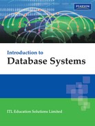
Whenever a transaction is submitted to a DBMS for execution, either it executes successfully or fails due to some reasons. During its execution, a transaction passes through various states that are active, partially committed, committed, failed, and aborted. Figure 9.1 shows the state transition diagram that describes how a transaction passes through various states during its execution.

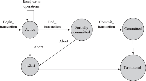
Fig. 9.1 State transition diagram showing various states of a transaction

A transaction enters into the active state with its commencement. At this point, the system marks BEGIN_TRANSACTION operation to specify the beginning of the transaction execution. During its execution, the transaction stays in the active state and executes several READ and WRITE operations on the database. The READ operation transfers a data item from the database to a local buffer of the transaction that has executed the read operation. The WRITE operation transfers the data item from the local buffer of the transaction back to the database.

Once the transaction executes its final operation, the system marks END_TRANSACTION operation to specify the end of the transaction execution. At this point, the transaction enters into partially committed state. The actual output at this point may still be residing in the main memory and thus, any kind of hardware failure might prevent its successful completion. In such a case, the transaction may have to be aborted.

Before actually updating the database on the disk, the system first writes the details of updates performed by the transaction in the log file (discussed in Chapter 11). The log file is then written to the disk so that, even in case of failure, the system can re-construct the updates performed by the transaction when the system restarts after the failure. When this information is successfully written out in the log file, the system marks COMMIT_TRANSACTION operation to indicate the successful end of the transaction. Now, the transaction is said to be committed and all its changes must be reflected permanently in the database.

If the transaction is aborted during its active state or the system fails to write the changes in log file, the transaction enters into the failed state. The failed transaction must be rolled back to undo its effects on the database to maintain the consistency of the database. When the transaction leaves the system, it enters into the terminated state. At this point, the transaction information maintained in the log file during its execution is removed.

An aborted transaction can be restarted either automatically or by the user. A transaction can only be restarted automatically by the system if it was aborted due to some hardware or software error and not due to some internal logical error of the transaction. If the transaction was aborted due to some internal logic error or because the desired data was not found in the database, then it must be killed by the database system. In this case, the user must first rectify the error in the transaction and then submit it again to the system as a new transaction for execution.

Note that once a transaction has been committed, its effects cannot be undone by aborting it. The only way to undo the effects of a committed transaction is to execute a compensating transaction, which reverses the effect of a committed transaction. For example, a transaction that has added $100 in an account can be reversed back by executing a compensating transaction that would subtract $100 from the account. However, it is not always possible to create a compensating transaction. Therefore, it is the responsibility of the user, and not of the database system, to write and execute a compensating transaction.

9.3 CONCURRENT EXECUTION OF TRANSACTIONS

The transaction-processing system allows concurrent execution of multiple transactions to improve the system performance. In concurrent execution, the database management system controls the execution of two or more transactions in parallel; however, allows only one operation of any transaction to occur at any given time within the system. This is also known as interleaved execution of multiple transactions. The database system allows concurrent execution of transactions due to two reasons.

First, a transaction performing read or write operation using I/O devices may not be using the CPU at a particular point of time. Thus, while one transaction is performing I/O operations, the CPU can process another transaction. This is possible because CPU and I/O system in the computer system are capable of operating in parallel. This overlapping of I/O and CPU activities reduces the amount of time for which the disks and processors are idle and, thus, increases the throughput of the system (the number of transactions executed in a given amount of time).

Second, interleaved execution of a short and a long transaction allows short transaction to complete quickly. If a short transaction is executed after the execution of a long transaction in a serial order, the short transaction may have to wait for a long time, leading to unpredictable delays in executing a transaction. On the other hand, if these transactions are executed concurrently, it reduces the unpredictable delays, and thereby reduces the average response time.

Note that despite the correctness of each individual transaction, undesirable interleaving of multiple transactions may lead to database inconsistency. Thus, interleaving should be done carefully to ensure that the result of a concurrent execution of transactions is equivalent to some serial execution (one after the other) of the same set of transactions. The database system must control the interaction among concurrently executing transactions. The database system does so with the help of several concurrency-control techniques which are discussed in Chapter 10.

9.3.1 Anomalies Due to Interleaved Execution

If the transactions are interleaved in an undesirable manner, it may lead to several anomalies such as lost update, dirty read, and unrepeatable read. To understand the effect of these anomalies on the database, consider two transactions T₁ and T₂, where T₁ transfers $100 from account A to account B, and T₂ adds two percent interest to account A. Suppose that the initial values of account A and B are $2000 and $1500, respectively. Then, after the serial execution of transactions T₁ and T₂ (T₁ followed by T₂), the value of account A should be $1938 and that of account B should be $1600.

Suppose that the operations of T₁ and T₂ are interleaved in such a way that T₂ reads the value of account A before T₁ updates its value in the database. Now, when T₂ updates the value of account A in the database, the value of account A updated by the transaction T₁ is overwritten and hence, is lost. This is known as lost update problem. The value of account A at the end of both the transactions is $2040 instead of $1938 which leads to data inconsistency. The interleaved execution of transactions T₁ and T₂ that leads to lost update problem is shown in Figure 9.2.

Fig. 9.2 Lost update problem

The second problem occurs when a transaction fails after updating a data item, and before this data item is changed back to its original value, another transaction reads this updated value. For example, assume that T₁ fails after debiting $100 from account A, but before crediting this amount to account B. This will leave the database in an inconsistent state. The value of account A is now $1900, which must be changed back to original one, that is, $2000. However, before the transaction T₁ is rolled back, let another transaction T₂ reads the incorrect value of account A. This incorrect value of account A that is read by transaction T₂ is called dirty data, and the problem is called dirty read problem. The interleaved execution of transactions T₁ and T₂ that leads to dirty read problem is shown in Figure 9.3.

Fig. 9.3 Dirty read problem

The third problem occurs when a transaction tries to read the value of the data item twice, and another transaction updates the same data item in between the two read operations of the first transaction. As a result, the first transaction reads varied values of same data item during its execution. This is known as unrepeatable read. For example, consider a transaction T₃ that reads the value of account A. At this point, let another transaction T₄ updates the value of account A. Now if T₃ again tries to read the value of account A, it will get a different value. As a result, the transaction T₃ receives different values for two reads of account A. The interleaved schedule of transactions T₃ and T₄ that leads to a problem of unrepeatable read is shown in Figure 9.4.

Fig. 9.4 Unrepeatable read

9.4 TRANSACTION SCHEDULES

A list of operations (such as reading, writing, aborting or committing) from a set of transactions is known as a schedule (or history). A schedule should comprise all the instructions of the participating transactions and also preserve the order in which the instructions appear in each individual transaction.

Consider two transactions T₁ and T₅, where T₁ transfers $100 from account A to account B and T₅ transfers $50 from account B to account C. Here, account C is another account of the shopkeeper. Suppose that the values of account A, B, and C are $2000, $1500, and $500, respectively. The sum A + B + C is $4000. Also suppose that the two transactions are executed one after the other in the order T₁ followed by T₅. Figure 9.5 shows the serial execution of transactions T₁ and T₅. This sequence of execution of the transactions is called a serial schedule. A serial schedule consists of a sequence of instructions from various transactions, where the operations of one single transaction appear together in that schedule. Hence, for a set of n transactions, n! different valid serial schedules are possible.

Fig. 9.5 Schedule 1—A serial schedule in the order T₁ followed by T₅

In Figure 9.5, the sequence of instructions is in chronological order from top to bottom with the instructions of transaction T₁ appearing in the left column followed by the instructions of T₅ appearing in the right column. The final values of accounts A, B, and C after the execution of both the transactions are $1900, $1550, and $550, respectively. The sum A + B + C is preserved after the execution of both the transactions.

Similarly, if the transaction T₁ is executed after the execution of transaction T₅, then also the sum A + B + C is preserved. The serial schedule of transactions T₁ and T₅ in the order T₅ followed by T₁ is shown in Figure 9.6.

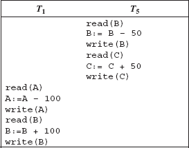
Fig. 9.6 Schedule 2—A serial schedule in the order T₅ followed by T₁

A schedule can also be described with the help of shorthand notation that uses the symbols r, w, c, and a, for the operations read, write, commit, and abort, respectively. Note that for the purpose of recovery and concurrency control, we are only interested in these four operations. The transaction id (transaction number) is also appended as a subscript to each operation in the schedule. For example, Schedule 1 of Figure 9.5, which may be named S₁, can be expressed as given here.

S1: r1(A); w1(A); r1(B); w1(B); r5(B); w5(B); r5(C); w5(C);

Each transaction in a serial schedule is executed independently without any interference from the operations of other transactions. As long as every transaction is executed from beginning to end without any interference from other transactions, it gives a correct end result on the database. Therefore, every serial schedule is considered to be correct. However, in serial schedules only one transaction is active at a time. The commit or abort operations of the active transaction initiates the next transaction. The transactions are not interleaved in a serial schedule. Thus, if the active transaction is waiting for an I/O operation, CPU cannot be used for another transaction, which results in CPU idle time. Moreover, if one transaction is quite long, the other transactions have to wait for long time for their turn. Hence, serial schedules are unacceptable.

9.4.1 Serializable Schedules

In a multi-user database system, several transactions are executed concurrently for efficient use of system resources. When two transactions are executed concurrently, the operating system may execute one transaction for some time, then perform a context switch and execute the second transaction for some time, and then switch back to the first transaction, and so on. Thus, when multiple transactions are executed concurrently, the CPU time is shared among all the transactions. The schedule resulted from this type of interleaving of operations from various transactions is known as non-serial schedule.

In general, there is no way to predict exactly how many operations of a transaction will be executed before the CPU switches to another transaction. Thus, for a set of n transactions, the number of possible non-serial schedules is much larger than n!. However, not all non-serial schedules result in the correct state of the database. For example, the schedule for the transactions T₁ and T₅ shown in Figure 9.7 is not a correct schedule as it leaves the database in an inconsistent state. After the execution of this schedule, the final values of accounts A, B, and C are $1900, $1600, and $550, respectively. Thus, the sum A + B + C is not preserved.

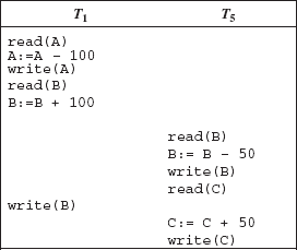
Fig. 9.7 Schedule 3—A concurrent schedule resulting in an inconsistent state of database

The consistency of the database under concurrent execution can be ensured by interleaving the operations of transactions in such a way that the final output is same as that of some serial schedule of those transactions. Such a schedule is referred to as serializable schedule. Thus, a schedule S of n transactions T₁, T₂, T₃, …, T_n is serializable if it is equivalent to some serial schedule of the same n transactions.

Figure 9.8 shows a non-serial schedule of transactions T₁ and T₅ which is equivalent to Schedule 1. After the execution of this schedule, the final values of accounts A, B, and C are $1900, $1550, and $550. Thus, the sum A + B + C is preserved and hence, it is a serializable schedule. The shorthand notation for this schedule is given here.

S4: r1(A); w1(A); r5(B); w5(B); r1(B); w1(B); r5(C); w5(C);

Fig. 9.8 Schedule 4—A concurrent schedule resulting in consistent state of the database

9.4.2 Schedules Equivalence

Two different schedules may produce the same final state of the database. Such schedules are known as result equivalent, since they have same effect on the database. However, in some cases, two different schedules may accidentally produce the same final state of database. For example, consider two schedules S_i and S_j that are updating the data item Q, as shown in the Figure 9.9.

Fig. 9.9 Schedules S_i and S_j

Suppose that value of data item Q is $100 then the final state of database produced by schedules S_i and S_j is same, that is, they produce the same value of Q ($200). However, if the initial value of data item Q is other than $100, the final state may not be the same. For example, if the initial value of Q is $200, then these schedules will not produce the same final state. Thus, with this initial value, the schedules S_i and S_j are not result equivalent. Moreover, these two schedules execute two different transactions and hence, cannot be considered as equivalent. Thus, result equivalence alone is not the sufficient condition for defining the equivalence of the schedules. Two other most commonly used forms of schedule equivalence are conflict equivalence and view equivalence that lead to the notions of conflict serializability and view serializability.

Conflict Equivalence and Conflict Serializability

Two operations in a schedule are said to conflict if they belong to different transactions, access the same data item, and at least one of them is the write operation. On the other hand, two operations belonging to different transactions in a schedule do not conflict if both of them are read operations or both of them are accessing different data items. To understand the concept of conflicting operations in a schedule, consider two transactions T₆ and T₇ that are updating the data items Q and R in the database. A non-serial schedule of these transactions is shown in Figure 9.10. Here, we have taken only read and write operations as these are the only significant operations from the scheduling point of view.

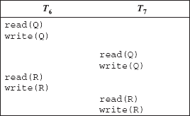
Fig. 9.10 Schedule 5—showing only read and write operations

In Schedule 5, the write(Q) operation of T₆ conflicts with the read(Q) operation of T₇ because both the operations are accessing the same data item Q, and one of these operations is the write operation. On the other hand, the write(Q) operation of T₇ is not conflicting with read(R) operation of T₆, because both are accessing different data items Q and R.

The order of execution of two conflicting operations is important because if they are applied in different order, they can have different effect on the database or on the other transactions in the schedule. For example, if write(Q) operation of T₆ is swapped with read(Q) operation of T₇, the value read by the read(Q) operation can be different. However, the order of execution of non-conflicting operations does not matter. It means that if write(Q) operation of T₇ is swapped with read(Q) operation of T₆, then a new schedule is produced, which will have the same effect on the database as Schedule 5. The equivalent schedule (Schedule 6) in which all the operations appear in the same order as that of the Schedule 5 except for the write(Q) and read(R) operations of T₇ and T₆, respectively is shown in Figure 9.11. Note that the schedules shown in Figures 9.10 and 9.11 produce the same final state of the database regardless of initial system state.

Fig. 9.11 Schedule 6 — after swapping nonconflicting operations of Schedule 5

Similarly, we can reorder the following non-conflicting operations in the Schedule 5, without affecting its impact on the database.

• read(R) operation of T₆ is swapped with read(Q) operation of T₇
• write(R) operation of T₆ is swapped with write(Q) operation of T₇
• write(R) operation of T₆ is swapped with read(Q) operation of T₇

The resultant schedule generated from the sequence of these steps is shown in Figure 9.12. Note that this schedule is a serial schedule. Thus, we have shown that Schedule 5 is equivalent to a serial schedule (Schedule 7). This equivalence means that regardless of the initial system state, Schedule 5 will produce the same final state as some serial schedule.

Fig. 9.12 Schedule 7—serial schedule equivalent to Schedule 5

If a schedule S can be transformed into a schedule S′ by performing a series of swaps of non-conflicting operations, then S and S′ are conflict equivalent. In other words, two schedules are said to be conflict equivalent if the order of any two conflicting operations is same in both the schedules. For example, Schedule 5 and Schedule 6 are conflict equivalent. The concept of conflict equivalence leads to the concept of conflict serializability. A schedule, which is conflict equivalent to some serial schedule, is known as conflict serializable. Hence, Schedule 5 is a conflict serializable schedule as it is conflict equivalent to a serial schedule (Schedule 7).

To better understand the concept of conflict equivalent and conflict serializable schedules, consider Schedule 8 and Schedule 9 of transactions T₈ and T₉ shown in Figure 9.13. The write(Q) operation of T₈ and read(Q) operation of T₉ are conflicting operations in both the schedules and the order of these operations in both the schedules is also same. Thus, Schedule 8 and Schedule 9 are conflict equivalent. Moreover, Schedule 9 is a serial schedule; hence, Schedule 8 is conflict serializable schedule.

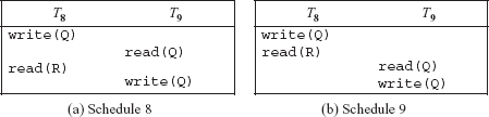
Fig. 9.13 Conflict serializable schedules

Testing Schedules for Conflict Serializability The conflict serializability of a schedule can be tested using a simple algorithm that considers only read and write operations in a schedule to construct a precedence graph (or serialization graph). A precedence graph is a directed graph G = (N,E) where N = {T₁, T₂, …, T_n} is a set of nodes and E = {e₁, e₂, …, e_n} is a set of directed edges. For each transaction T_i in a schedule, there exists a node in the graph. An edge e_i in the graph is shown as (T_i → T_j), where T_i is the starting node and T_j is the ending node of the edge e_i. The edge e_i is created if one of the operations in T_j appears in the schedule before some conflicting operation in T_j.

The algorithm to test the conflict serializability of a schedule S is given here.

1. For each transaction T_i participating in the schedule S, create a node labelled T_i.
2. If T_j executes a read operation after T_iexecutes a write operation on any data item say Q, create an edge (T_i → T_j) in the precedence graph.
3. If T_j executes a write operation after T_i executes a read operation on any data item say Q, create an edge (T_i → T_j) in the precedence graph.
4. If T_j executes a write operation after T_i executes a write operation on any data item say Q, create an edge (T_i→ T_j) in the precedence graph.
5. If the resultant precedence graph is acyclic, that is, it does not contain any cycle, then the schedule S is considered to be conflict serializable. If a precedence graph contains a cycle, the schedule S is not conflict serializable.

Some examples of cyclic and acyclic precedence graphs are shown in Figure 9.14. Note that the edges (T_i → T_j) in a precedence graph can also be labelled by the name of the data item that led to the creation of the edge (see Figure 9.15).

Fig. 9.14 Acyclic and cyclic precedence graphs

An edge from T_i to T_j in the precedence graph implies that the transaction T_i must appear before T_j in any serial schedule S′ that is equivalent to S. Thus, if there are no cycles in the precedence graph, a serial schedule S′ equivalent to S can be created by ordering the transactions in such a way that whenever an edge (T_i → T_j) exists in the precedence graph, T_i must appear before T_j in the equivalent serial schedule S′. The process of ordering the nodes of an acyclic preceding graph is known as topological sorting. The topological ordering produces equivalent serial schedule.

For example, consider Schedule 5 shown in Figure 9.10. The precedence graph of this schedule is shown in Figure 9.15(a). The precedence graph contains two nodes, one for each transaction—T₆ and T₇. An edge from T₆ to T₇ is created which is labelled with the data items Q and R that led to the creation of this edge. Since there are no cycles in the precedence graph, Schedule 5 is conflict serializable schedule. The serial schedule equivalent to Schedule 5 is shown in Figure 9.15(b).

Fig. 9.15 An example of testing conflict serializability

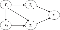
Though only one serial schedule exists for Schedule 5, in general, there can be more than one equivalent serial schedule for a conflict serializable schedule. For example, consider a precedence graph for a schedule of three transactions T₁, T₂, and T₃ shown in Figure 9.16(a). It has two equivalent serial schedules shown in Figure 9.16(b).

Fig. 9.16 Precedence graph with two equivalent schedules

To better understand the concept of testing a conflict serializability of a schedule, consider Schedule 10 of three transactions T₁₀, T₁₁, and T₁₂ shown in Figure 9.17(a). In this schedule, the read(Q) operation of T₁₀ and write(Q) operation of T₁₂ are the conflicting operations. Similarly, the write(Q) operation of T₁₂ and read(Q) operation of T₁₁ are the conflicting operations. The write(R) operation of T₁₁ and read(R) operation of T₁₀ are also conflicting operations. Thus, a precedence graph with edges from T₁₀ to T₁₂, T₁₂ to T₁₁, and T₁₁ to T₁₀ is created [see Figure 9.17(b)]. Since this graph contains cycle (T₁₀ → T₁₂ → T₁₁ → T₁₀), the Schedule 10 is not conflict serializable. Therefore, no serial schedule equivalent to this schedule will exist.

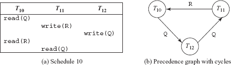
Fig. 9.17 Schedule 10 and its precedence graph

View Equivalence and View Serializability

Equivalence of schedules can also be determined by another less restrictive definition of equivalence called view equivalence. Two schedules S and S′ are said to be view equivalent if the schedules satisfy these conditions.

1. The same set of transactions participates in S and S′, and S and S′ include the same set of operations of those transactions.
2. If the transaction T_i reads the initial value of a data item say Q in schedule S, then T_i must read the initial value of same data item Q in schedule S′ also.
3. For each data item Q, if T_i executes read(Q) operation after the write(Q) operation of transaction T_j in schedule S, then T_i must execute the read(Q) operation after the write(Q) operation of T_j in schedule S′ also.
4. If the transaction T_i performs the final write operation on any data item say Q in schedule S, then it must perform final write operation on the same data item Q in schedule S′ also.

Conditions 2 and 3 ensure that as long as each transaction reads the same values in both the schedules, they perform the same computation. Conditions 4 (along with conditions 2 and 3) ensure that the final write operation on each data item is same in both the schedules and hence, produces the same final state of the database. The concept of view equivalence leads to the concept of view serializability. A schedule S is said to be view serializable if it is view equivalent to some serial schedule.

Fig. 9.18 View serializable schedules

To better understand the concept of view equivalence and view serializability, consider Schedule 11 and Schedule 12 of three transactions T₁₃, T₁₄, and T₁₅ shown in Figure 9.18. In both these schedules, the transaction T₁₄ reads the initial value of data item Q (condition 2). Moreover, in both the schedules, the transaction T₁₃ performs the read(R) operation after the write(R) operation of T₁₄ (condition 3). Similarly, the transaction T₁₅ performs read(R) operation after the write(R) operation of T₁₄ in both the schedules. Finally, in both the schedules, the transaction T₁₅ performs the final write(Q) operation (condition 4). Thus, Schedule 11 and Schedule 12 are view equivalent. Moreover, Schedule 12 is a serial schedule hence, Schedule 11 is view serializable also.

Now, consider Schedule 13 given in Figure 9.19. In this schedule, the transactions T₁₇ and T₁₈ perform write(Q) operation without performing the read(Q) operation. Thus, the value written by the write(Q) operation is independent of the old value of Q in the database. These types of write operations are known as blind writes. This schedule is view equivalent to some serial schedule of transactions T₁₆, T₁₇, and T₁₈. Hence, it is view serializable. However, it is not conflict serializable since its precedence graph is cyclic (see Figure 9.20). Thus, blind writes appear in a view serializable schedule that is not conflict serializable.

 

Fig. 9.19 Schedule 13—showing an example of blind write

Fig. 9.20 Precedence graph of Schedule 13

9.4.3 Recoverable and Cascadeless Schedules

The computer systems are prone to failures. Hence, it is important to consider the effects of transaction failure during concurrent execution. As discussed earlier, if a transaction T_i fails due to any reason; its effects need to be undone to ensure atomicity property of the transaction. During concurrent execution of transactions, it must be ensured that any transaction T_j that depends on T_i (that is, T_j has read the value of data item written by T_i) must also be rolled back. Thus, some restrictions must be placed on the type of schedules permitted in the system.

Two types of schedules, namely, recoverable and cascadeless schedules are acceptable from the viewpoint of recovery from transaction failure. If, in a schedule S, a transaction T_j reads a data item written by T_i, then the commit operation of T_i should appear before the commit operation of T_j. Such a schedule is known as recoverable schedule.

Consider Schedule 14 of transactions T₁₉ and T₂₀ as shown in the Figure 9.21. The transaction T₂₀ performs read(Q) operation after the write(Q) operation of T₁₉. Suppose that immediately after read(Q) operation, transaction T₂₀ commits. Now if transaction T₁₉ fails, its effects need to be undone in order to ensure atomicity of the transaction. Since, T₂₀ has read the value of Q written by T₁₉, it also has to be rolled back. However, T₂₀ has already been committed, thus, cannot be rolled back. In such situations, it becomes impossible to recover from the failure of transaction T₁₉. Such schedules are known as non-recoverable schedule s. The database system must ensure that the schedules are recoverable. If the commit operation of transaction T₂₀ in Figure 9.21 is performed after the commit operation of T₁₉, the schedule becomes recoverable.

Fig. 9.21 Schedule 14

Sometimes, even if a schedule is recoverable, several transactions may have to be rolled back in order to recover completely from the failure of a transaction T_i. It happens if transactions have read the value of a data item written by T_i. For example, consider Schedule 15 shown in Figure 9.22. In this schedule, the transaction T₂₂ reads the value of data item Q written by transaction T₂₁, and transaction T₂₃ reads the value of data item Q written by transaction T₂₂.

Fig. 9.22 Schedule 15

Now suppose that the transaction T₂₁ fails due to any reason, it has to be rolled back. Since transaction T₂₂ has read the data written by T₂₁, it also needs to be rolled back. The transaction T₂₃ also needs to be rolled back because it has in turn read the data written by T₂₂. Such a situation, in which failure of a single transaction leads to a series of transaction rollbacks, is called cascading rollback.

Cascading rollback requires undoing of significant amount of work and thus, is undesirable. Therefore, schedules should be restricted to avoid cascading rollbacks. The schedules that avoid cascading rollbacks are known as cascadeless schedule. In cascadeless schedules, transactions T_i and T_j are interleaved in such a way that T_j reads a data item previously written by T_i; however, commit operation of T_i appears before the read operation of T_j.

 

9.5 SQL TRANSACTION STATEMENTS

As discussed earlier that the statements of a transaction are enclosed within the begin transaction and end transaction statements. However, in SQL:92 standard, there is no explicit BEGIN TRANSACTION statement. A transaction initiates implicitly when SQL statements are encountered. However, an explicit end statement is required which can be COMMIT or ROLLBACK statement. Execution of a COMMIT statement or ROLLBACK statement completes the current transaction.

The COMMIT statement terminates the current transaction and makes all the changes made by the transaction permanent in the database. That is, it commits the changes to the database. The COMMIT statement has the following general format.

COMMIT [WORK]

where,

WORK is an optional keyword that does not change the semantics of COMMIT

The ROLLBACK statement, on the other hand, terminates the current transaction and undoes all the changes made by the transaction. That is, it rolls back the changes to the database. The ROLLBACK statement has the following general format.

ROLLBACK [WORK]

In this case also, WORK is an optional keyword that does not change the semantics of ROLLBACK.

9.5.1 Transaction Characteristics in SQL

Every transaction in SQL has certain characteristics associated with it such as access mode, diagnostic area size, and isolation level. The SET TRANSACTION statement in SQL:92 is used to specify these characteristics. The access mode can be specified as READ ONLY or READ WRITE. The READ ONLY mode allows only retrieval of data from the database. The READ WRITE mode, on the other hand, allows UPDATE, INSERT, DELETE, and CREATE commands to be executed.

The diagnostic area size option, specified as DIAGNOSTIC SIZE n, determines the number of error or exception conditions that can be recorded in the diagnostic area for the current transaction. The diagnostic area is populated for each SQL statement that is executed. If the statement raised more conditions than the specified DIAGNOSTIC SIZE, only most severe conditions will be reported. For example, if we specify DIAGNOSTIC SIZE 5 but one of the SQL statements raised 10 conditions, it is most likely that only “most severe” 5 conditions will be reported.

SQL:92 also supports four levels of transaction isolation. The isolation levels reduce the isolation between concurrently executing transactions. The level providing the greatest isolation from other transactions is SERIALIZABLE. It is the default level of isolation. At this level, a transaction is fully isolated from the changes made by other transactions. The other isolation levels are READ UNCOMMITTED, READ COMMITTED, and REPEATABLE READ. READ UNCOMMITTED is the lowest level of isolation. At this level, a transaction can read subsequent changes made by other transactions, either committed or uncommitted. With read uncommitted isolation level, one or more of the three problems, namely, dirty read, unrepeatable read, and phantom read may occur.

We have already discussed the dirty read and unrepeatable read problems. Phantom read problem occurs when a transaction T_i reads a set of rows from a table based on some condition specified in WHERE clause, meanwhile another transaction T_j inserts a new row into that table that also satisfies the condition and commits. Now, if T_i is again executed, then it will see a tuple (or phantom tuple) that previously did not exist.

The next level above READ UNCOMMITTED is READ COMMITTED, and above that is REPEATABLE READ. In READ COMMITTED isolation level, dirty reads are not possible since a transaction is not allowed to read the updates made by uncommitted transactions. However, unrepeatable reads and phantoms are possible. In REPEATABLE READ isolation level, dirty reads and unrepeatable reads are not possible but phantoms are possible. In SERIALIZABLE isolation level, dirty reads, unrepeatable reads, and phantoms are not possible. The possible violations for different transaction isolation levels are summarized in Table 9.1.

 

Table 9.1 Possible violations for different isolation levels

An example of an SQL transaction consisting of multiple SQL statements is given in Figure 9.23. In this transaction, two SQL statements are given that update the BOOK and PUBLISHER relations of Online Book database. The first statement updates the price of all the books published by publisher P001. The next statement updates the email-id of the publisher with P_ID=“P002”. If an error occurs on any SQL statement, the entire transaction is rolled back. That is, any updated value would be restored to its original value.

 

	EXEC	SQL WHENEVER SQLERROR GOTO mylabel;
	EXEC	SQL SET TRANSACTION READ WRITE, ISOLATION LEVEL SERIALIZABLE, DIAGNOSTIC SIZE 10;
	EXEC	SQL UPDATE BOOK SET Price=Price*1.2 WHERE P_ID=“P001”;
	EXEC	SQL UPDATE PUBLISHER SET Email_id=“[email protected]” WHERE P_ID=“P002”;
	EXEC	SQL COMMIT;
	GOTO	LAST;
	mylabel:	EXEC SQL ROLLBACK;
	LAST:…;

 

Fig. 9.23 An example of SQL transaction

1. A collection of operations that form a single logical unit of work is called a transaction. The statements of a transaction are enclosed within the begin transaction and end transaction statements.
2. For a transaction to be completed and database changes to be made permanent, a transaction has to be completed in its entirety.
3. To ensure the integrity of the data, the database system must maintain some desirable properties of the transaction. These properties are known as ACID properties, the acronym derived from the first letter of the terms atomicity, consistency, isolation, and durability.
4. Atomicity implies that either all of the operations that make up a transaction should execute or none of them should occur.
5. Consistency implies that if all the operations of a transaction are executed completely without the interference of other transactions, the consistency of the database is preserved.
6. Isolation implies that each transaction appears to run in isolation with other concurrently running transactions.
7. Durability (also known as permanence) implies that once a transaction is completed successfully, the changes made by the transaction persist, even if the system fails.
8. Whenever a transaction is submitted to a DBMS for execution, either it executes successfully or fails due to some reasons. During its execution, a transaction passes through various states such as active, partially completed, committed, failed, and aborted.
9. The transaction-processing system allows concurrent execution of multiple transactions to improve the system performance.
10. In concurrent execution, the database management system controls the execution of two or more transactions in parallel; however, allows only one operation of any transaction to occur at any given time within the system. This is also known as interleaved execution of multiple transactions.
11. The undesirable interleaved execution of transactions may lead to certain problems such as lost update, dirty read, and unrepeatable read.
12. A list of operations (such as reading, writing, aborting, or committing) from a set of transaction is known as a schedule (or history). A schedule should comprise all the instructions of the participating transactions and also preserve the order in which the instructions appear in each individual transaction.
13. A serial schedule consists of a sequence of instructions from various transactions, where the operations of one single transaction appear together in that schedule.
14. The consistency of the database under concurrent execution can be ensured by interleaving the operations of transactions in such a way that the final output is same as that of some serial schedule of those transactions. Such a schedule is referred to as serializable schedule.
15. There are several ways to define schedule equivalence. The simplest way of defining schedule equivalence is to compare the result of the schedules on the database. Two schedules are known as result equivalent if they produce same final state of the database.
16. Two other most commonly used forms of schedule equivalence are conflict equivalence and view equivalence that lead to the notions of conflict serializability and view serializability.
17. Two operations in a schedule are said to conflict if they belong to different transactions, access the same data item and at least one of them is write operation.
18. Two schedules are said to be conflict equivalent if the order of any two conflicting operations is same in both the schedules. A schedule, which is conflict equivalent to some serial schedule, is known as conflict serializable.
19. The conflict serializability of a schedule can be tested using a simple algorithm that considers only read and write operations in a schedule to construct a precedence graph. A precedence graph is a directed graph consists of a set of nodes and a set of directed edges.
20. If the precedence graph is acyclic then the schedule is considered to be conflict serializable. If a precedence graph contains a cycle, the schedule is not conflict serializable.
21. The process of ordering the nodes of an acyclic preceding graph is known as topological sorting.
22. Equivalence of schedules can also be determined by another less restrictive definition of equivalence called view equivalence. A schedule S is said to be view serializable if it is view equivalent to some serial schedule.
23. The computer systems are prone to failure. Hence, it is important to consider the effects of transaction failure during concurrent execution.
24. A situation, in which failure of single transaction leads to a series of transaction rollbacks, is called cascading rollback. The database system must ensure that the schedules are recoverable and cascadeless.

• ACID properties
• Atomicity
• Consistency
• Isolation
• Durability
• Active state
• Read-only transaction
• Partially committed state
• Committed transaction
• Failed state
• Terminated state
• Compensating transaction
• Interleaved execution
• Throughput
• Lost update
• Dirty read
• Unrepeatable read
• Schedule
• Serial schedule
• Non-serial schedule
• Serializable schedule
• Result equivalent schedules
• Conflict serializability
• View serializability
• Conflict
• Conflict equivalent schedules
• Conflict serializable schedules
• Precedence graph (or serialization graph)
• Topological sorting
• View equivalent schedules
• View serializable schedules
• Blind writes
• Recoverable schedule
• Non-recoverable schedule
• Cascading rollback
• Cascadeless schedule
• Begin transaction statement
• End transaction statement
• Access mode
• Diagnostic area size
• Isolation levels
• Phantom read problem

A. Multiple Choice Questions

1. What does C stand for in transaction ACID properties?
   1. Correctness
   2. Consistency
   3. Committed
   4. Completeness
2. Once the transaction executes its final operation, it enters into _______________ state.
   1. Committed
   2. Terminated
   3. Partially committed
   4. Failed
3. The only way to undo the effects of a committed transaction is to execute a ______________.
   1. Undo transaction
   2. Compensating transaction
   3. Redo transaction
   4. None of these
4. Why is concurrent execution of transactions preferred over serial execution?
   1. To increase system throughput
   2. To decrease average response time
   3. Both (a) and (b)
   4. None of these
5. Which of these anomalies is also known as WW conflict?
   1. Lost update
   2. Dirty read
   3. Unrepeatable read
   4. None of these
6. Which of these operations is considered for the purpose of recovery and concurrency control?
   1. Write
   2. Commit
   3. Abort
   4. All of these
7. How many valid serial schedules are possible for four transactions?
   1. 24
   2. 16
   3. 4
   4. 8
8. Two schedules are known as ______________ if they produce same final state of the database.
   1. Serializable
   2. Conflict equivalent
   3. Result equivalent
   4. View equivalent
9. The schedules that avoid cascading rollbacks are known as ___________________.
   1. Cascadeless schedules
   2. Recoverable schedules
   3. Serial schedules
   4. Non-recoverable schedules
10. How many levels of transaction isolation does SQL:92 support?
    1. Two
    2. Three
    3. Four
    4. Five

B. Fill in the Blanks

1. ____________ implies that once a transaction is completed successfully, the changes made by the transaction persist in the database, even if the system fails.
2. If the transaction is aborted during its active state or the system fails to write the changes in log file, the transaction enters into the ________ state.
3. If the transactions are interleaved in an undesirable manner, it may lead to several anomalies such as ___________, ___________, and ____________.
4. The interleaving of the operations of transactions in such a way that the final output is same as that of some serial schedule of those transactions is known as ______________.
5. Two schedules are known as _____________ if they produce same final state of the database.
6. Two operations in a schedule are said to ____________ if they belong to different transactions, access the same data item and at least one of them is write operation.
7. A schedule, which is conflict equivalent to some serial schedule, is known as ____________.
8. The process of ordering the nodes of an acyclic preceding graph is known as ____________.
9. A schedule S is said to be _____________ if it is view equivalent to some serial schedule.
10. A situation, in which failure of single transaction leads to a series of transaction rollbacks, is called _____________.

C. Answer the Questions

1. What is a transaction? What are ACID properties of a transaction? Violation of which property causes lost update problem? Justify with the help of an example.
2. What are the two main operations that a transaction uses to access data from the database?
3. What do you mean by state transition diagram? When a transaction is said to be failed, explain with the help of an example.
4. Why is it important to interleave multiple transactions? Discuss the various anomalies that can occur due to undesirable interleaving of transactions. Give suitable examples also.
5. Define the following terms:
   1. Schedule
   2. Non-serial schedule
   3. Topological sorting
   4. Average response time
   5. Observable external writes
   6. Cascading rollback
   7. Blind writes
6. What is a serial schedule? Why is it always considered to be correct?
7. What is a serializable schedule? Give an example also.
8. When two schedules are result equivalent? Explain with example.
9. Discuss the two different forms of schedule equivalence. Give the steps to test the conflict serializability of a schedule S.
10. What is a precedence graph?
11. Every cascadeless schedule is also recoverable. Justify this statement by taking suitable example.
12. Discuss the four levels of isolation in SQL. What are the possible violations for these levels?

D. Practical Questions

1. Consider two transactions T₁ and T₂ given below:

   T1	T2
   read(X)	read(X)
   X:=X-10	X:=X*1.02
   write(X)	Y:=Y*1.02
   read(Y)	write(X)
   Y:=Y+10	write(Y)
   write(Y)

   Give a serial schedule for these transactions and an equivalent non-serial schedule for these transactions.

2. Consider the following precedence graph. Is the corresponding schedule is conflict serializable? Give reasons also.
   
3. Consider three transactions T₁, T₂, and T₃ and two schedules S₁ and S₂ given below. Draw the precedence graph for schedules S₁ and S₂ and test whether they are conflict serializable or not.

    

   T1: r1(P); r1(R); w1(P);

   T2: r2(R); r2(Q); w2(R); w2(Q);

   T1: r3(P); r3(Q); w3(Q);

   S1: r1(P); r2(R); r1(R); r3(P); r3(Q); w1(P); w3(Q); r2(Q); w2(R); w2(Q);

   S2: r1(P); r2(R); r3(P); r1(R); r2(Q); r3(Q); w1(P); w2(R); w3(Q); w2(Q);

    

4. Consider schedule S₃ given below. Determine whether it is cascadeless, recoverable, or non-recoverable.

    

   S3: r1(P); r2(R); r1(R); r3(P); r3(Q); w1(P); w3(Q); r2(Q); w3(R); w2(Q); c1; c2; c3

    

5. Give an example of SQL transaction.