1. Risk Management and Financial Returns
This chapter begins by listing the learning objectives of the book. We then discuss theoretical reasons for why firms should spend resources on risk management and discuss the empirical evidence of the effectiveness and impact of current risk management practices in the corporate and financial sectors. Next, we list the types of risks faced by a corporation, and we briefly discuss the costs and benefits of exposure to each type of risk. The chapter also develops a list of stylized facts of asset returns, which a proper risk model needs to capture. Finally, we introduce the Value-at-Risk concept for risk measurement.
Keywords: Types of risk, asset returns, stylized facts of returns, Value-at-Risk.
1. Chapter Outline
This chapter begins by listing the learning objectives of the book. We then ask why firms should be occupied with risk management in the first place. In answering this question, we discuss the apparent contradiction between standard investment theory and the emergence of risk management as a field, and we list theoretical reasons why managers should give attention to risk management. We also discuss the empirical evidence of the effectiveness and impact of current risk management practices in the corporate as well as financial sectors. Next, we list a taxonomy of the potential risks faced by a corporation, and we briefly discuss the desirability of exposure to each type of risk. After the risk taxonomy discussion, we define asset returns and then list the stylized facts of returns, which are illustrated by the S&P 500 equity index. We then introduce the Value-at-Risk concept. Finally, we present an overview of the remainder of the book.
2. Learning Objectives
The book is intended as a practical handbook for risk managers as well as a textbook for students. It suggests a relatively sophisticated approach to risk measurement and risk modeling. The idea behind the book is to document key features of risky asset returns and then construct tractable statistical models that capture these features. More specifically, the book is structured to help the reader
• Become familiar with the range of risks facing corporations and learn how to measure and manage these risks. The discussion will focus on various aspects of market risk.
• Become familiar with the salient features of speculative asset returns.
• Apply state-of-the-art risk measurement and risk management techniques, which are nevertheless tractable in realistic situations.
• Use derivatives in risk management.
• Understand the current academic and practitioner literature on risk management techniques.
3. Risk Management and the Firm
Before diving into the discussion of the range of risks facing a corporation and before analyzing the state-of-the art techniques available for measuring and managing these risks it is appropriate to start by asking the basic question about financial risk management.
3.1. Why Should Firms Manage Risk?
From a purely academic perspective, corporate interest in risk management seems curious. Classic portfolio theory tells us that investors can eliminate asset-specific risk by diversifying their holdings to include many different assets. As asset-specific risk can be avoided in this fashion, having exposure to it will not be rewarded in the market. Instead, investors should hold a combination of the risk-free asset and the market portfolio, where the exact combination will depend on the investor's appetite for risk. In this basic setup, firms should not waste resources on risk management, since investors do not care about the firm-specific risk.
From the celebrated Modigliani-Miller theorem, we similarly know that the value of a firm is independent of its risk structure; firms should simply maximize expected profits, regardless of the risk entailed; holders of securities can achieve risk transfers via appropriate portfolio allocations. It is clear, however, that the strict conditions required for the Modigliani-Miller theorem are routinely violated in practice. In particular, capital market imperfections, such as taxes and costs of financial distress, cause the theorem to fail and create a role for risk management. Thus, more realistic descriptions of the corporate setting give some justifications for why firms should devote careful attention to the risks facing them:
• Bankruptcy costs. The direct and indirect costs of bankruptcy are large and well known. If investors see future bankruptcy as a nontrivial possibility, then the real costs of a company reorganization or shutdown will reduce the current valuation of the firm. Thus, risk management can increase the value of a firm by reducing the probability of default.
• Taxes. Risk management can help reduce taxes by reducing the volatility of earnings. Many tax systems have built-in progressions and limits on the ability to carry forward in time the tax benefit of past losses. Thus, everything else being equal, lowering the volatility of future pretax income will lower the net present value of future tax payments and thus increase the value of the firm.
• Capital structure and the cost of capital. A major source of corporate default is the inability to service debt. Other things equal, the higher the debt-to-equity ratio, the riskier the firm. Risk management can therefore be seen as allowing the firm to have a higher debt-to-equity ratio, which is beneficial if debt financing is inexpensive net of taxes. Similarly, proper risk management may allow the firm to expand more aggressively through debt financing.
• Compensation packages. Due to their implicit investment in firm-specific human capital, managerial level and other key employees in a firm often have a large and unhedged exposure to the risk of the firm they work for. Thus, the riskier the firm, the more compensation current and potential employees will require to stay with or join the firm. Proper risk management can therefore help reduce the costs of retaining and recruiting key personnel.
3.2. Evidence on Risk Management Practices
A while ago, researchers at the Wharton School surveyed 2000 companies on their risk management practices, including derivatives uses. Of the 2000 firms surveyed, 400 responded. Not surprisingly, the survey found that companies use a range of methods and have a variety of reasons for using derivatives. It was also clear that not all risks that were managed were necessarily completely removed. About half of the respondents reported that they use derivatives as a risk-management tool. One-third of derivative users actively take positions reflecting their market views, thus they may be using derivatives to increase risk rather than reduce it.
Of course, not only derivatives are used to manage risky cash flows. Companies can also rely on good old-fashioned techniques such as the physical storage of goods (i.e., inventory holdings), cash buffers, and business diversification.
Not everyone chooses to manage risk, and risk management approaches differ from one firm to the next. This partly reflects the fact that the risk management goals differ across firms. In particular, some firms use cash-flow volatility, while others use the variation in the value of the firm as the risk management object of interest. It is also generally found that large firms tend to manage risk more actively than do small firms, which is perhaps surprising as small firms are generally viewed to be more risky. However, smaller firms may have limited access to derivatives markets and furthermore lack staff with risk management skills.
3.3. Does Risk Management Improve Firm Performance?
The overall answer to this question appears to be yes. Analysis of the risk management practices in the gold mining industry found that share prices were less sensitive to gold price movements after risk management. Similarly, in the natural gas industry, better risk management has been found to result in less variable stock prices. A study also found that risk management in a wide group of firms led to a reduced exposure to interest rate and exchange rate movements.
Although it is not surprising that risk management leads to lower variability—indeed the opposite finding would be shocking—a more important question is whether risk management improves corporate performance. Again, the answer appears to be yes.
Researchers have found that less volatile cash flows result in lower costs of capital and more investment. It has also been found that a portfolio of firms using risk management would outperform a portfolio of firms that did not, when other aspects of the portfolio were controlled for. Similarly, a study found that firms using foreign exchange derivatives had higher market value than those who did not.
The evidence so far paints a fairly rosy picture of the benefits of current risk management practices in the corporate sector. However, evidence on the risk management systems in some of the largest US commercial banks is less cheerful. Several recent studies have found that while the risk forecasts on average tended to be overly conservative, perhaps a virtue at certain times, the realized losses far exceeded the risk forecasts. Importantly, the excessive losses tended to occur on consecutive days. Thus, looking back at the data on the a priori risk forecasts and the ex ante loss realizations, we would have been able to forecast an excessive loss tomorrow based on the observation of an excessive loss today. This serial dependence unveils a potential flaw in current financial sector risk management practices, and it motivates the development and implementation of new tools such as those presented in this book.
4. A Brief Taxonomy of Risks
We have already mentioned a number of risks facing a corporation, but so far we have not been precise regarding their definitions. Now is the time to make up for that.
Market risk is defined as the risk to a financial portfolio from movements in market prices such as equity prices, foreign exchange rates, interest rates, and commodity prices.
While financial firms take on a lot of market risk and thus reap the profits (and losses), they typically try to choose the type of risk to which they want to be exposed. An option trading desk, for example, has a lot of exposure to volatility changing, but not to the direction of the stock market. Option traders try to be delta neutral, as it is called. Their expertise is volatility and not market direction, and they only take on the risk about which they are the most knowledgeable, namely volatility risk. Thus financial firms tend to manage market risk actively. Nonfinancial firms, on the other hand, might decide that their core business risk (say chip manufacturing) is all they want exposure to and they therefore want to mitigate market risk or ideally eliminate it altogether.
Liquidity risk is defined as the particular risk from conducting transactions in markets with low liquidity as evidenced in low trading volume and large bid-ask spreads. Under such conditions, the attempt to sell assets may push prices lower, and assets may have to be sold at prices below their fundamental values or within a time frame longer than expected.
Traditionally, liquidity risk was given scant attention in risk management, but the events in the fall of 2008 sharply increased the attention devoted to liquidity risk. The housing crisis translated into a financial sector crises that rapidly became an equity market crisis. The flight to low-risk treasury securities dried up liquidity in the markets for risky securities. The 2008–2009 crisis was exacerbated by a withdrawal of funding by banks to each other and to the corporate sector. Funding risk is often thought of as a type of liquidity risk.
Operational risk is defined as the risk of loss due to physical catastrophe, technical failure, and human error in the operation of a firm, including fraud, failure of management, and process errors.
Operational risk (or op risk) should be mitigated and ideally eliminated in any firm because the exposure to it offers very little return (the short-term cost savings of being careless, for example). Op risk is typically very difficult to hedge in asset markets, although certain specialized products such as weather derivatives and catastrophe bonds might offer somewhat of a hedge in certain situations. Op risk is instead typically managed using self-insurance or third-party insurance.
Credit risk is defined as the risk that a counterparty may become less likely to fulfill its obligation in part or in full on the agreed upon date. Thus credit risk consists not only of the risk that a counterparty completely defaults on its obligation, but also that it only pays in part or after the agreed upon date.
The nature of commercial banks traditionally has been to take on large amounts of credit risk through their loan portfolios. Today, banks spend much effort to carefully manage their credit risk exposure. Nonbank financials as well as nonfinancial corporations might instead want to completely eliminate credit risk because it is not part of their core business. However, many kinds of credit risks are not readily hedged in financial markets, and corporations often are forced to take on credit risk exposure that they would rather be without.
Business risk is defined as the risk that changes in variables of a business plan will destroy that plan's viability, including quantifiable risks such as business cycle and demand equation risk, and nonquantifiable risks such as changes in competitive behavior or technology. Business risk is sometimes simply defined as the types of risks that are an integral part of the core business of the firm and therefore simply should be taken on.
The risk taxonomy defined here is of course somewhat artificial. The lines between the different kinds of risk are often blurred. The securitization of credit risk via credit default swaps (CDS) is a prime example of a credit risk (the risk of default) becoming a market risk (the price of the CDS).
5. Asset Returns Definitions
While any of the preceding risks can be important to a corporation, this book focuses on various aspects of market risk. Since market risk is caused by movements in asset prices or equivalently asset returns, we begin by defining returns and then give an overview of the characteristics of typical asset returns. Because returns have much better statistical properties than price levels, risk modeling focuses on describing the dynamics of returns rather than prices.
The daily continuously compounded or log return on an asset is instead defined as
The two definitions of return convey the same information but each definition has pros and cons. The simple rate of return definition has the advantage that the rate of return on a portfolio is the portfolio of the rates of return. Let Ni be the number of units (for example shares) held in asset i and let VPF,t be the value of the portfolio on day t so that
Most assets have a lower bound of zero on the price. Log returns are more convenient for preserving this lower bound in the risk model because an arbitrarily large negative log return tomorrow will still imply a positive price at the end of tomorrow. When using log returns tomorrow's price is
If we instead use the rate of return definition then tomorrow's closing price is
Another advantage of the log return definition is that we can easily calculate the compounded return at the K–day horizon simply as the sum of the daily returns:
This book will use the log return definition unless otherwise mentioned.
6. Stylized Facts of Asset Returns
We can now consider the following list of so-called stylized facts—or tendencies—which apply to most financial asset returns. Each of these facts will be discussed in detail in the book. The statistical concepts used will be explained further in Chapter 3. We will use daily returns on the S&P 500 from January 1, 2001, through December 31, 2010, to illustrate each of the features.
Daily returns have very little autocorrelation. We can write

The unconditional distribution of daily returns does not follow the normal distribution. Figure 1.2 shows a histogram of the daily S&P 500 return data with the normal distribution imposed. Notice how the histogram is more peaked around zero than the normal distribution. Daily returns tend to have more small positive and fewer small negative returns than the normal distribution. Although the histogram is not an ideal graphical tool for analyzing extremes, extreme returns are also more common in daily returns than in the normal distribution. We say that the daily return distribution has fat tails. Fat tails mean a higher probability of large losses (and gains) than the normal distribution would suggest. Appropriately capturing these fat tails is crucial in risk management.

The stock market exhibits occasional, very large drops but not equally large up-moves. Consequently, the return distribution is asymmetric or negatively skewed. Some markets such as that for foreign exchange tend to show less evidence of skewness.
The standard deviation of returns completely dominates the mean of returns at short horizons such as daily. It is not possible to statistically reject a zero mean return. Our S&P 500 data have a daily mean of 0.0056% and a daily standard deviation of 1.3771%.
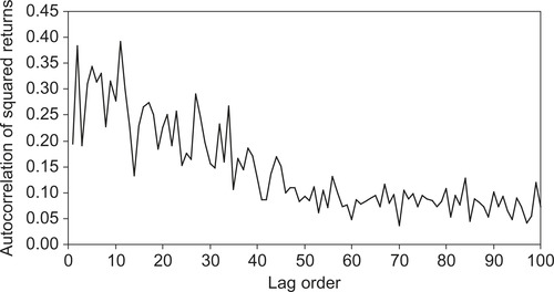
Variance, measured, for example, by squared returns, displays positive correlation with its own past. This is most evident at short horizons such as daily or weekly. Figure 1.3 shows the autocorrelation in squared returns for the S&P 500 data, that is
Equity and equity indices display negative correlation between variance and returns. This is often called the leverage effect, arising from the fact that a drop in a stock price will increase the leverage of the firm as long as debt stays constant. This increase in leverage might explain the increase in variance associated with the price drop. We will model the leverage effect in Chapter 4 and Chapter 5.
Correlation between assets appears to be time varying. Importantly, the correlation between assets appears to increase in highly volatile down markets and extremely so during market crashes. We will model this important phenomenon in Chapter 7.
Even after standardizing returns by a time-varying volatility measure, they still have fatter than normal tails. We will refer to this as evidence of conditional nonnormality, which will be modeled in Chapter 6 and Chapter 9.
As the return-horizon increases, the unconditional return distribution changes and looks increasingly like the normal distribution. Issues related to risk management across horizons will be discussed in Chapter 8.
7. A Generic Model of Asset Returns
Based on the previous list of stylized facts, our model of individual asset returns will take the generic form
In most of the book, we will assume that the conditional mean of the return, μt + 1, is simply zero. For daily data this is a quite reasonable assumption as we mentioned in the preceding list of stylized facts. For longer horizons, the risk manager may want to estimate a model for the conditional mean as well as for the conditional variance. However, robust conditional mean relationships are not easy to find, and assuming a zero mean return may indeed be the most prudent choice the risk manager can make.
Chapter 4 and Chapter 5 will be devoted to modeling σt + 1. For now we can simply rely on JP Morgan's RiskMetrics model for dynamic volatility. In that model, the volatility for tomorrow, time t + 1, is computed at the end of today, time t, using the following simple updating rule:
8. From Asset Prices to Portfolio Returns
Consider a portfolio of n assets. The value of a portfolio at time t is again the weighted average of the asset prices using the current holdings of each asset as weights:
Having defined the portfolio return we are ready to introduce one of the most commonly used portfolio risk measures, namely Value-at-Risk.
9. Introducing the Value-at-Risk (VaR) Risk Measure
Value-at-Risk, or VaR, is a simple risk measure that answers the following question: What loss is such that it will only be exceeded p · 100% of the time in the next Ktrading days? VaR is often defined in dollars, denoted by $VaR, so that the $VaR loss is implicitly defined from the probability of getting an even larger loss as in
This book builds models for log returns and so we will instead use a VaR based on log returns defined as
So now the −VaR is defined as the number so that we would get a worse log return only with probability p. That is, we are (1 − p) 100% confident that we will get a return better than −VaR. This is the definition of VaR we will be using throughout the book. When writing the VaR in return terms it is much easier to gauge its magnitude. Knowing that the $VaR of a portfolio is $500,000 does not mean much unless we know the value of the portfolio. Knowing that the return VaR is 15% conveys more relevant information. The appendix to this chapter shows that the two VaRs are related via
If we start by considering a very simple example, namely that our portfolio consists of just one security, for example an S&P 500 index fund, then we can use the RiskMetrics model to provide the VaR for the portfolio. Let  denote the p · 100% VaR for the 1-day ahead return, and assume that returns are normally distributed with zero mean and standard deviation σPF, t + 1. Then

Φ(z) calculates the probability of being below the number z, and  instead calculates the number such that p · 100% of the probability mass is below
  . Taking Φ−1(*) on both sides of the preceding equation yields the VaR as

Because  is always negative for p < 0.5, the negative sign in front of the VaR formula again ensures that the VaR itself is a positive number. The interpretation is thus that the VaR gives a number such that there is a 1% chance of losing more than 5.825% of the portfolio value today. If the value of the portfolio today is $2 million, the $VaR would simply be
Figure 1.4 illustrates the VaR from a normal distribution. Notice that we assume that K = 1 and p = 0.01 here. The top panel shows the VaR in the probability distribution function, and the bottom panel shows the VaR in the cumulative distribution function. Because we have assumed that returns are normally distributed with a mean of zero, the VaR can be calculated very easily. All we need is a volatility forecast.

VaR has undoubtedly become the industry benchmark for risk calculation. This is because it captures an important aspect of risk, namely how bad things can get with a certain probability, p. Furthermore, it is easily communicated and easily understood.
VaR does, however, have drawbacks. Most important, extreme losses are ignored. The VaR number only tells us that 1% of the time we will get a return below the reported VaR number, but it says nothing about what will happen in those 1% worst cases. Furthermore, the VaR assumes that the portfolio is constant across the next K days, which is unrealistic in many cases when K is larger than a day or a week. Finally, it may not be clear how K and p should be chosen. Later we will discuss other risk measures that can improve on some of the shortcomings of VaR.
As another simple example, consider a portfolio whose value consists of 40 shares in Microsoft (MS) and 50 shares in GE. A simple way to calculate the VaR for the portfolio of these two stocks is to collect historical share price data for MS and GE and construct the historical portfolio pseudo returns using
We can now directly model the volatility of the portfolio return, RPF, t + 1, call it σPF, t + 1, and then calculate the VaR for the portfolio as

Notice that this aggregate VaR method is directly dependent on the portfolio positions (40 shares and 50 shares), and it would require us to redo the volatility modeling every time the portfolio is changed or every time we contemplate change and want to study the impact on VaR of changing the portfolio allocations. Although modeling the aggregate portfolio return directly may be appropriate for passive portfolio risk measurement, it is not as useful for active risk management. To do sensitivity analysis and assess the benefits of diversification, we need models of the dependence between the return on individual assets or risk factors. We will consider univariate, portfolio-level risk models in Part II of the book and multivariate or asset level risk models in Part III of the book.
We also hasten to add that the assumption of normality when computing VaR is made for convenience and is not realistic. Important methods for dealing with the nonnormality evident in daily returns will be discussed in Chapter 6 of Part II (univariate nonnormality) and in Chapter 9 of Part III (multivariate nonnormality).
10. Overview of the Book
The book is split into four parts and contains a total of 13 chapters including this one.
Part I, which includes Chapter 2 and Chapter 3, contains various background material on risk management. Chapter 1 has discussed the motivation for risk management and listed important stylized facts that the risk model should capture. Chapter 2 introduces the Historical Simulation approach to Value-at-Risk and discusses the reasons for going beyond the Historical Simulation approach when measuring risk. Chapter 2 also compares the Value-at-Risk and Expected Shortfall risk measures. Chapter 3 provides a primer on the basic concepts in probability and statistics used in financial risk management. It can be skipped by readers with a strong statistical background.
Part II of the book includes Chapter 4, Chapter 5 and Chapter 6 and develops a framework for risk measurement at the portfolio level. All the models introduced in Part II are univariate. They can be used to model assets individually or to model the aggregate portfolio return. Chapter 4 discusses methods for estimating and forecasting time-varying daily return variance using daily data. Chapter 5 uses intraday return data to model and forecast daily variance. Chapter 6 introduces methods to model the tail behavior in asset returns that is not captured by volatility models and that is not captured by the normal distribution.
Part III includes Chapter 7, Chapter 8 and Chapter 9 and it covers multivariate risk models that are capable of aggregating asset level risk models to provide sensible portfolio level risk measures. Chapter 7 introduces dynamic correlation models, which together with the dynamic volatility models in Chapter 4 and Chapter 5 can be used to construct dynamic covariance matrices for many assets. Chapter 9 introduces copula models that can be used to aggregate the univariate distribution models in Chapter 6 and thus provide proper multivariate distributions. Chapter 8 shows how the various models estimated on daily data can be used via simulation to provide estimates of risk across different investment horizons.
Part IV of the book includes Chapter 10, Chapter 11, Chapter 12 and Chapter 13 and contains various further topics in risk management. Chapter 10 develops models for pricing options when volatility is dynamic. Chapter 11 discusses the risk management of portfolios that include options. Chapter 12 discusses credit risk management. Chapter 13 develops methods for backtesting and stress testing risk models.
Appendix. Return VaR and $VaR
This appendix shows the relationship between the return VaR using log returns and the $VaR. First, the unknown future value of the portfolio is VPFexp (RPF) where VPF is the current market value of the portfolio and RPF is log return on the portfolio. The dollar loss $Loss is simply the negative change in the portfolio value and so the relationship between the portfolio log return RPF and the $Loss is
Further Resources
A very nice review of the theoretical and empirical evidence on corporate risk management can be found in Stulz (1996) and Damodaran (2007).
For empirical evidence on the efficacy of risk management across a range of industries, see Allayannis and Weston (2003), Cornaggia (2010), MacKay and Moeller (2007), Minton and Schrand (1999), Purnanandam (2008), Rountree et al. (2008), Smithson (1999) and Tufano (1998).
Berkowitz and O'Brien (2002), Perignon and Smith, 2010a and Perignon and Smith, 2010b and Perignon et al. (2008) document the performance of risk management systems in large commercial banks, and Dunbar (1999) contains a discussion of the increased focus on risk management after the turbulence in the fall of 1998.
The definitions of the main types of risk used here can be found at www.erisk.com and in JPMorgan/Risk Magazine (2001).
The stylized facts of asset returns are provided in Cont (2001). Surveys of Value-at-Risk models include Andersen et al. (2006), Basle Committee for Banking Supervision (2011), Christoffersen (2009), Duffie and Pan (1997), Kuester et al. (2006) and Marshall and Siegel (1997).
Useful web sites include www.gloriamundi.org, www.risk.net, www.defaultrisk.com and www.bis.org. See also www.christoffersen.com.
Allayannis, G., Weston, J., 2003. Earnings Volatility, Cash-Flow Volatility and Firm Value. Manuscript, University of Virginia, Charlottesville, VA and Rice University, Houston, TX.
Andersen, T.G.; Bollerslev, T.; Christoffersen, P.F.; Diebold, F.X., Practical Volatility and Correlation Modeling for Financial Market Risk Management, In: (Editors: Carey, M.; Stulz, R.) (2006) The NBER Volume on Risks of Financial Institutions, University of Chicago Press, Chicago, IL.
Basle Committee for Banking Supervision, 2011. Messages from the Academic Literature on Risk Measurement for the Trading Book. Basel Committee on Banking Supervision, Working Paper, Basel, Switzerland.
Berkowitz, J.; O'Brien, J., How accurate are Value-at-Risk models at commercial banks?J. Finance 57 (2002) 1093–1112.
Christoffersen, P.F., Value-at-Risk models, In: (Editors: Andersen, T.G.; Davis, R.A.; Kreiss, J.-P.; Mikosch, T.) Handbook of Financial Time Series (2009) Springer Verlag, Düsseldorf, Germany.
Cont, R., Empirical properties of asset returns: Stylized facts and statistical issues, Quant. Finance 1 (2001) 223–236.
Cornaggia, J., Does Risk Management Matter?. (2010) Manuscript, Indiana University, Bloomington, IN.
Damodaran, A., Strategic Risk Taking: A Framework for Risk Management. (2007) Wharton School Publishing, Pearson Education, Inc. Publishing as Prentice Hall, Upper Saddle River, NY.
Duffie, D.; Pan, J., An overview of Value-at-Risk, J. Derivatives 4 (1997) 7–49.
Dunbar, N., The new emperors of Wall Street, Risk (1999) 26–33.
JPMorgan/Risk Magazine, Guide to Risk Management: A Glossary of Terms. (2001) Risk Waters Group, London.
Kuester, K.; Mittnik, S.; Paolella, M.S., Value-at-Risk prediction: A comparison of alternative strategies, J. Financial Econom. 4 (2006) 53–89.
MacKay, P.; Moeller, S.B., The value of corporate risk management, J. Finance 62 (2007) 1379–1419.
Marshall, C.; Siegel, M., Value-at-Risk: Implementing a risk measurement standard, J. Derivatives 4 (1997) 91–111.
Minton, B.; Schrand, C., The impact of cash flow volatility on discretionary investment and the costs of debt and equity financing, J. Financial Econom. 54 (1999) 423–460.
Perignon, C.; Deng, Z.; Wang, Z., Do banks overstate their Value-at-Risk?J. Bank. Finance 32 (2008) 783–794.
Perignon, C.; Smith, D., The level and quality of Value-at-Risk disclosure by commercial banks, J. Bank. Finance 34 (2010) 362–377.
Perignon, C.; Smith, D., Diversification and Value-at-Risk, J. Bank. Finance 34 (2010) 55–66.
Purnanandam, A., Financial distress and corporate risk management: Theory and evidence, J. Financial Econom. 87 (2008) 706–739.
Rountree, B.; Weston, J.P.; Allayannis, G., Do investors value smooth performance?J. Financial Econom. 90 (2008) 237–251.
Smithson, C., Does risk management work?Risk (1999) 44–45.
Stulz, R., Rethinking risk management, J. Appl. Corp. Finance 9 (1996) 8–24.
Tufano, P., The determinants of stock price exposure: Financial engineering and the gold mining industry, J. Finance 53 (1998) 1015–1052.
Open the Chapter1Data.xlsx file on the web site. (Excel hint: Enable the Data Analysis Tool under Tools, Add-Ins.)
1. From the S&P 500 prices, remove the prices that are simply repeats of the previous day's price because they indicate a missing observation due to a holiday. Calculate daily log returns as Rt + 1 = ln(St + 1) − ln(St) where St + 1 is the closing price on day t + 1, St is the closing price on day t, and ln (*) is the natural logarithm. Plot the closing prices and returns over time.
2. Calculate the mean, standard deviation, skewness, and kurtosis of returns. Plot a histogram of the returns with the normal distribution imposed as well. (Excel hints: You can either use the Histogram tool under Data Analysis, or you can use the functions AVERAGE, STDEV, SKEW, KURT, and the array function FREQUENCY, as well as the NORMDIST function. Note that KURT computes excess kurtosis.)
3. Calculate the first through 100th lag autocorrelation. Plot the autocorrelations against the lag order. (Excel hint: Use the function CORREL.) Compare your result with Figure 1.1.
4. Calculate the first through 100th lag autocorrelation of squared returns. Again, plot the autocorrelations against the lag order. Compare your result with Figure 1.3.
5. Set  (i.e., the variance of the first observation) equal to the variance of the entire sequence of returns (you can square the standard deviation found earlier). Then calculate
  for t = 2, 3, …, T (the last observation). Plot the sequence of standard deviations (i.e., plot σt).
6. Compute standardized returns as zt = Rt/σt and calculate the mean, standard deviation, skewness, and kurtosis of the standardized returns. Compare them with those found in exercise 2.
7. Calculate daily, 5-day, 10-day, and 15-day nonoverlapping log returns. Calculate the mean, standard deviation, skewness, and kurtosis for all four return horizons. Do the returns look more normal as the horizon increases?
8. Calculate the 1-day, 1% VaR on each day in the sample using the sequence of variances  and the standard normal distribution assumption for the shock zt + 1.
The answers to these exercises can be found in the Chapter1Results.xlsx file on the companion site.
For more information see the companion site at http://www.elsevierdirect.com/companions/9780123744487
..................Content has been hidden....................
You can't read the all page of ebook, please click here login for view all page.