
7. Covariance and Correlation Models
The objective of this chapter is to model the linear dependence, or correlation, between returns on different assets. Correlation models will enable us to calculate risk measures on portfolios of securities such as stocks, bonds, and foreign exchange rates for many different combinations of portfolio weights. We first present a general model of portfolio risk for large-dimensional portfolios with many assets and then consider ways to reduce the problem of dimensionality. The main challenge of the chapter is modeling the dynamic aspects of correlation. We will consider dynamic correlation models of varying degrees of sophistication, both in terms of their specification and of the information required to calculate them.
Keywords: Covariance, correlation, factor structure, DCC models, realized covariance.
1. Chapter Overview
Chapter 4, Chapter 5 and Chapter 6 covered various aspects of modeling the aggregate portfolio return. The univariate methods in those chapters can also be used to model the return on each individual asset. Chapter 8 and Chapter 9 will cover multivariate risk models. They will enable us to join together the univariate asset level models in Chapter 4, Chapter 5 and Chapter 6.
Although modeling the aggregate portfolio return directly is useful for passive portfolio risk measurement, it is not as useful for active risk management. In order to perform sensitivity analysis (for example, what happens to my portfolio risk if I buy another share of IBM?) and in order to assess the benefits of diversification, we need models of the dependence between the return on individual assets. We will proceed on this front in three steps. Chapter 7 (the present chapter) will model dynamic covariance and correlation, which together with the dynamic volatility models in Chapter 4 and Chapter 5 can be used to construct covariance matrices. Chapter 8 will develop some important simulation tools such as Monte Carlo and bootstrapping, which are needed for multiperiod risk assessments. Chapter 9 will introduce copula models, which can be used to link together the nonnormal univariate distributions in Chapter 6. Correlation models only allow for linear dependence between asset returns whereas copula models allow for nonlinear dependence.
The objective of this chapter is to model the linear dependence, or correlation, between returns on different assets, such as IBM and Microsoft stocks, or on different classes of assets, such as stock indices and foreign exchange (FX) rates. Once this is done, we will be able to calculate risk measures on portfolios of securities such as stocks, bonds, and foreign exchange rates for many different combinations of portfolio weights.
We first present a general model of portfolio risk for large-dimensional portfolios with many assets and consider ways to reduce the problem of dimensionality. Just as the main topic of the previous chapter was modeling the dynamic aspects of variance, the main topic of this chapter is modeling the dynamic aspects of correlation. We then consider dynamic correlation models of varying degrees of sophistication, both in terms of their specification and of the information required to calculate them.
Just as Chapter 4 and Chapter 5 temporarily assumed the univariate normal distribution in order to focus on volatility modeling, in this chapter we will assume the multivariate normal distribution for the purpose of covariance and correlation modeling. We hasten to add that the assumption of multivariate normality is made for convenience and is not realistic. Important methods for dealing with the multivariate nonnormality evident in daily returns will be discussed in Chapter 8 and Chapter 9.
2. Portfolio Variance and Covariance
We now establish some notation that is necessary to study the risk of portfolios consisting of an arbitrary number of securities, n. The return on the portfolio on day t + 1 is defined as
For daily log returns the portfolio return relationship will hold approximately
Chapter 4, Chapter 5 and Chapter 6 modeled the univariate  time series (or
  ), Chapter 8 and Chapter 9 will model the multivariate time series
  ,
,  (or
(or  ). The models we will develop later for dynamic covariance and correlation can equally well be used for log returns and rates of returns, but
  ,
,  , and
, and  computations that depend on the portfolio weights,
  will only be exact when we use the rate of return definition,
  .
.
The variance of the portfolio can be written as
Using vector notation, we will write

If we are willing to assume that returns are multivariate normal, then the portfolio return, which is just a linear combination of asset returns, will be normally distributed, and we have
Notice that even if we have already constructed volatility forecasts for each of the securities in the portfolio, then we still have to model and forecast all the correlations. If we have n assets, then we will have n(n − 1)/2 different correlations, so if n is 100, then we'll have 4950 correlations to model, which would be a daunting task. We will therefore explicitly be looking for methods that are able to handle large-dimensional portfolios.
2.1. Exposure Mappings
A very simple way to reduce the dimensionality of the portfolio variance is to impose a factor structure using observed market returns as factors. In the extreme case we may be able to assume that the portfolio return is just the (systematic) market return plus a portfolio specific (idiosyncratic) risk term as in
The portfolio variance in this case is
In the case of a very well diversified stock portfolio, for example, it may be reasonable to assume that the variance of the portfolio equals that of the S&P 500 market index. In this case, only one volatility—that of the S&P 500 index return—needs to be modeled, and no correlation modeling is necessary. This is referred to as index mapping and can be written as
The 1-day VaR assuming normality is simply
More generally, in portfolios that contain systematic risk, we have
If the portfolio is well diversified so that systematic market risk explains a large part of the variation in the portfolio return then the portfolio-specific idiosyncratic risk can be ignored, and we can pose a linear relationship between the portfolio and the market index and use the so-called beta mapping, as in
Finally, the risk manager of a large-scale portfolio may consider risk as mainly coming from a reasonable number of factors nF where nF < < n so that we have many fewer risk factors than assets. The exact choice of factors depends highly on the particular portfolio at hand, but they could be, for example, country equity indices, FX rates, or commodity price indices. Let us assume that we need 10 factors. We can write the 10-factor return model as
In this case, it makes sense to model the variances and correlations of these risk factors and assign exposures to each factor to get the portfolio variance. The portfolio variance in this general factor structure can be written
2.2. GARCH Conditional Covariances
Suppose the portfolio under consideration contains n assets. Alternatively, we can think of the risk manager as having chosen nF risk factors to be the main drivers of the risk in the portfolio. In either case, a covariance matrix must be estimated. To simplify notation, let us assume that we need an n-dimensional covariance matrix where n is 10 or larger. In portfolios with relatively few assets n will be the number of assets and in portfolios with many assets n will be the number of risk factors. We will refer to the assets or risk factors generically as “assets” in the following.
We now turn to various methods for constructing the time-varying covariance matrix Σt + 1. Arguably the simplest way to model time-varying covariances is to rely on plain rolling averages, a method that we considered for volatility in Chapter 4. For the covariance between asset (or risk factor) i and j, we can simply estimate
 |
| Figure 7.1 |
In order to avoid equal weighting we can instead use a simple exponential smoother model on the covariances, and let
 |
| Figure 7.2 |
The caveats that applied to the exponential smoother volatility model in Chapter 4 apply to the exponential smoother covariance model as well. The restriction that the coefficient (1 − λ) on the cross product of returns  and the coefficient
  on the past covariance
  sum to one is not necessarily desirable. It implies that there is no mean-reversion in covariance. Consider two highly correlated assets. If the forecast for tomorrow's covariance happens to be low today, then the forecast will be low for all future horizons in the exponential smoother model. The forecast from the model will not revert back to its (higher) mean when the horizon increases.
We can instead consider models with mean-reversion in covariance. For example, a GARCH-style specification for covariance would be
Notice that so far we have not allowed the persistence parameters λ in RiskMetrics and α and β in GARCH to vary across pairs of securities in the covariance models. This is no coincidence. It must be done to guarantee that the portfolio variance will be positive regardless of the portfolio weights, wt. We will say that a covariance matrix Σt + 1 is internally consistent if for all possible vectors wt of portfolio weights we have
This corresponds to saying that the covariance matrix is positive semidefinite. It is ensured by estimating volatilities and covariances in an internally consistent fashion. For example, relying on exponential smoothing using the same λ for every volatility and every covariance will work. Similarly, using a GARCH(1,1) model with α and β identical across variances and covariances and with long-run variances and covariances estimated consistently will work as well.
Unfortunately, it is not clear that the persistence parameters λ, α, and β should be the same for all variances and covariance. We therefore next consider methods that are not subject to this restriction.
3. Dynamic Conditional Correlation (DCC)
We now turn to the modeling of correlation rather than covariance. This is motivated by the desire to free up the restriction that variances and covariance have the same persistence parameters. We also want to assess if the time-variation in covariances arises solely from time-variation in the volatilities or if correlation has its own dynamic pattern. There is ample empirical evidence that correlations increase during financial turmoil and thereby increase risk even further; therefore, modeling correlation dynamics is crucial to a risk manager.
From Chapter 3, correlation is defined from covariance and volatility by
If, for example, we have the RiskMetrics model, then
The definition of correlation can be rearranged to provide the decomposition of covariance into volatility and correlation
We will consider the volatilities of each asset to already have been estimated through GARCH or one of the other methods considered in Chapter 4 and Chapter 5. We can then standardize each return by its dynamic standard deviation to get the standardized returns,

3.1. Exponential Smoother Correlations
We first consider simple exponential smoothing correlation models. Let the correlation dynamics be driven by  , which gets updated by the cross product of the standardized returns zi, t and zj, t as in
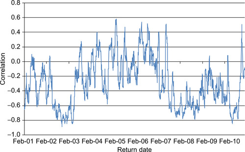
Figure 7.3 shows the exponential smoothed DCC correlations for the S&P 500 and 10-year treasury note example. Notice the dramatic changes in correlation over time.
 |
| Figure 7.3 |
The DCC model requires estimation of λ and we will discuss estimation in detail later.
3.2. Mean-Reverting Correlation
Just as we did for volatility and covariance models, we may want to consider a generalization of the exponential smoothing correlation model, which allows for correlations to revert to a long-run average correlation,  . We can consider GARCH(1,1)-type specifications of the form
The key thing to note about this model is that the correlation persistence parameters α and β are common across i and j. Thus, the model implies that the persistence of the correlation between any two assets in the portfolio is the same. It does not, however, imply that the level of the correlations at any time are the same across pairs of assets. The level of correlation is controlled by  and will thus vary over i and j. It does also not imply that the persistence in correlation is the same as the persistence in volatility. The persistence in volatility can vary from asset to asset, and it can vary from the persistence in correlation between the assets. But the model does imply that the persistence in correlation is constant across assets. Figure 7.4 shows the GARCH(1,1) correlations for the S&P 500 and 10-year treasury note example.
 |
| Figure 7.4 |
We can write the DCC models in matrix notation as

An important feature of these models is that the matrix Qt + 1 is positive semidefinite since it is a weighted average of positive semidefinite and positive definite matrices. This will in turn ensure that the correlation matrix  and the covariance matrix Σt + 1 will be positive semidefinite as required.
Another important practical advantage of the DCC model is that we can estimate the parameters in a sequential fashion. First, all the individual variances are estimated one by one using one of the methods from Chapter 4 and Chapter 5. Second, the returns are standardized and the unconditional correlation matrix is estimated. Third, the correlation persistence parameters α and β are estimated. The key issue is that only very few parameters are estimated simultaneously using numerical optimization. This feature makes the dynamic correlation models considered here extremely tractable for risk management of large portfolios. We now turn to the details of the estimation procedure.
3.3. Bivariate Quasi Maximum Likelihood Estimation
Fortunately, in estimating the dynamic conditional correlation models suggested earlier, we can rely on the quasi maximum likelihood estimation (QMLE) method, which we used for estimating the GARCH volatility models in Chapter 4.
Although a key benefit of the correlation models suggested here is that they are easy to estimate even for large portfolios, we will begin by analyzing the case of a portfolio consisting of only two assets. In this case, we can use the bivariate normal distribution function for z1, t and z2, t to write the log likelihood as

We find the optimal correlation parameter(s), in this case λ, by maximizing the correlation log-likelihood function, ln(Lc, 12). To initialize the dynamics, we set  and
and 
Notice that the variables that enter the likelihood are the standardized returns,  and not the original raw returns, Rt themselves. We are essentially treating the standardized returns as actual observations here.
As before, the QMLE method will give us consistent but inefficient estimates. In theory, we could obtain more precise results by estimating all the volatility models and the correlation model simultaneously. In practice, this is not feasible for large portfolios. In realistic situations, we are forced to rely on a stepwise QMLE method where we first estimate the volatility model for each of the assets and second estimate the correlation models. This approach gives decent parameter estimates while avoiding numerical optimization in high dimensions.
In the case of the mean-reverting GARCH correlations we have the same likelihood function and correlation definition but now

3.4. Composite Likelihood Estimation in Large Systems
In the general case of n assets in the portfolio, we typically have to rely on the n–dimensional normal distribution function to write the log likelihood as
Fortunately a very simple solution to this dimensionality problem is available in the DCC model. Rather than maximizing the n-dimensional log likelihood we can maximize the sum of the bivariate likelihoods

Computationally this composite likelihood function is much easier to maximize than the likelihood function where the n-dimensional correlation matrix must be inverted numerically. Note that rather than using all the available bivariate likelihoods in ln(CLc) we could just use a subset of them. The more we use the more precise our estimates will get.
3.5. An Asymmetric Correlation Model
So far we have considered only symmetric correlation models where the effect of two positive shocks is the same as the effect of two negative shocks of the same magnitude. But, just as we modeled the asymmetry in volatility (the leverage effect), we may want to allow for a down-market effect in correlation. This can be achieved using the asymmetric DCC model where
Note that γ corresponds to a leverage effect in correlation: When γ is positive then the correlation for asset i and j will increase more when zi, t and zj, t are negative than in any other case. If we envision a scatterplot of zi, t and zj, t, then γ > 0 will provide an extra increase in correlation when we observe an observation in the lower-left quadrant of the scatterplot. This captures a phenomenon often observed in markets for risky assets: Their correlation increases more in down markets (zi, t and zj, t both negative) than in up markets (zi, t and zj, t both positive). The basic DCC model does not directly capture this down-market effect but the asymmetric DCC model does.
4. Estimating Daily Covariance from Intraday Data
In Chapter 5 we considered methods for daily volatility estimation and forecasting that made use of intraday data. These methods can be extended to covariance estimation as well. When constructing RVs in Chapter 5 our biggest concern was biases arising from illiquidity effects: bid–ask bounces for example would bias upward our RV measure if we constructed intraday returns at a frequency that is too high.
The main concern when computing realized covariance is not bid–ask bounces but rather the asynchronicity of intraday prices across assets. Asynchronicity of intraday prices will cause a bias toward zero of realized covariance unless we estimate it carefully. Because asset covariances are typically positive a bias toward zero means we will be underestimating covariance and thus underestimating portfolio risk. This is clearly not a mistake we want to make.
4.1. Realized Covariance
Consider first daily covariance estimation using, say, 1-minute returns. As in Chapter 5, let the j th observation on day t + 1 for asset 1 be denoted  Then the j th return on day t + 1 is
However, from Chapter 5 we quickly realize that using the All RV estimate based on all m intraday returns is not a good idea because of the biases arising from illiquidity at high frequencies. We can instead rely on the Average (Avr) RV estimator, which averages across a number of sparse (using lower-frequency returns) RVs. Using the averaging idea for the RCov as well we would then have
Going from All RV to Average RV will fix the bias problems in the RV estimates but it will unfortunately not fix the bias in the RCov estimates: Asynchronicity will still cause a bias toward zero in RCov.
The current best practice for alleviating the asynchronicity bias in daily RCov relies on changing the time scale of the intraday observations. When we observe intraday prices on n assets the prices all arrive randomly throughout the day and randomly across assets. The trick for dealing with asynchronous data is to synchronize them using so-called refresh times.
Let τ (1) be the first time point on day t + 1 when all assets have changed their price at least once since market open. Let τ (2) be the first time point on day t + 1 when all assets have changed their price at least once since τ (1), and so on for  ,
,  The synchronized intraday returns for the n assets can now be computed using the τ (j) time points. For assets 1 and 2 we have
If realized variances are computed from the same refresh grid of prices
The synchronized RV and RCov estimates can be further refined by correcting for autocorrelation in the cross products of intraday returns as we did for RV in Chapter 5.
The RCov and RV measures can be used to build multivariate models for forecasting covariance and correlation. Some of the relevant references are listed at the end of the chapter.
4.2. Range-Based Covariance Using No-Arbitrage Conditions
Aside from the important synchronization problems, it is relatively straightforward to generalize the idea of realized volatility to realized correlation. However, extending range-based volatility to range-based correlation is not obvious because the cross product of the ranges does not capture covariance.
However, sometimes asset prices are linked together by no-arbitrage restrictions, and if so then range-based covariance can be constructed. Consider, for example, the case where S1 is the US$/yen FX rate, and S2 is the Euro/US$ FX rate. If we define S3to be the Euro/yen FX rate, then by ruling out arbitrage opportunities, we can write
Similar arbitrage arguments can be made between spot and futures prices and between portfolios and individual assets assuming of course that the range prices can be found on all the involved series.
Finally, as we suggested for volatility in Chapter 5, range-based proxies for covariance can be used as regressors in GARCH covariance models. Consider, for example,
Including the range-based covariance estimate in a GARCH model instead of using it by itself will have the beneficial effect of smoothing out some of the inherent noise in the range-based estimate of covariance.
Summary
Risk managers who want to calculate risk measures such as Value-at-Risk and Expected Shortfall for different portfolio allocations need to construct the matrix of variances and covariances for potentially large sets of assets. If returns are assumed to be normally distributed with a mean of zero, then the covariance matrix is all that is needed to calculate the VaR. This chapter thus considered methods for constructing the covariance matrix. First, we presented simple rolling estimates of covariance, followed by simple exponential smoothing and GARCH models of covariance. We then discussed the important issue of estimating variances and covariances in an internally consistent way so as to ensure that the covariance matrix is positive semidefinite and therefore generates sensible portfolio variances for all possible portfolio weights. This discussion led us to consider modeling the conditional correlation rather than the conditional covariance. We presented a simple framework for dynamic correlation modeling, which is based on standardized returns and which thus relies on preestimated volatility models such as those discussed in Chapter 4 and Chapter 5. Finally, methods for daily covariance and correlation estimation that make use of intraday information were introduced.
Further Resources
The choice of risk factors may be obvious for some portfolios, but in general it is not. It is therefore useful to let the return data help when deciding on what the factors should look like and how many factors we need. The choice of factors in a variety of portfolios is discussed in detail in Connor et al. (2010). A nice overview of the mechanics of assigning risk factor exposures can be found in Jorion (2006).
Bollerslev et al. (1988), Bollerslev (1990), Bollerslev and Engle (1993) and Engle and Kroner (1995) are some classic references on the first generation of multivariate GARCH models. See also the recent survey in Bauwens et al. (2006).
The conditional correlation model in this chapter is developed in Engle (2002), Engle and Sheppard (2001) and Tse and Tsui (2002). Aielli (2009) derives a refinement to the QMLE DCC estimation procedure described in this chapter. Cappiello et al. (2006) and Hafner and Franses (2009) develop extensions and alternatives to the basic DCC model. Composite likelihood estimation of DCC models is suggested in Engle et al. (2009). For a large-scale application of DCC models to international equity markets see Christoffersen et al. (2011).
Asynchronicity in returns is not just an issue in intraday data. It can also be a problem in daily returns for illiquid assets or for assets from markets that close at different times of the day. Burns et al. (1998) and Audrino and Buhlmann (2004) develop vector ARMA methods to deal with biases in correlation. Scholes and Williams (1977) use measurement error models to analyze bias of the beta estimate in the market model when daily closing prices are stale.
The construction of realized covariances is detailed in Barndorff-Nielsen et al. (2011), which also contains useful information on the cleaning of intraday data. Forecasting models using realized covariance and correlation are built in Bauer and Vorkink (2011), Chiriac and Voev (2011), Hansen et al. (2010), Jin and Maheu (2010), Voev (2008) and Noureldin et al. (2011).
Range-based covariance estimation is considered in Brandt and Diebold (2006), who also discuss ways to ensure positive semidefiniteness of the covariance matrix. Foreign exchange covariances estimated from intraday returns are reported in Andersen et al. (2001).
Finally, methods for the evaluation of covariance and correlation forecasts can be found in Patton and Sheppard (2009).
Aielli, G., Dynamic conditional correlations: On properties and estimation, Available from: SSRN,http://ssrn.com/abstract=1507743 (2009).
Andersen, T.; Bollerslev, T.; Diebold, F., The distribution of realized exchange rate volatility, J. Am. Stat. Assoc. 96 (2001) 42–55.
Audrino, F.; Buhlmann, P., Synchronizing multivariate financial time series, J. Risk 6 (2004) 81–106.
Barndorff-Nielsen, O.; Hansen, P.; Lunde, A.; Shephard, N., Multivariate realised kernels: Consistent positive semi-definite estimators of the covariation of equity prices with noise and non-synchronous trading, J. Econom. (2011); forthcoming.
Bauer, G.H.; Vorkink, K., Forecasting multivariate realized stock market volatility, J. Econom. 160 (2011) 93–101.
Bauwens, L.; Laurent, S.; Rombouts, J., Multivariate GARCH models: A survey, J. Appl. Econom. 21 (2006) 79–109.
Bollerslev, T., Modeling the coherence in short-run nominal exchange rates: A multivariate generalized ARCH model, Rev. Econ. Stat. 72 (1990) 498–505.
Bollerslev, T.; Engle, R., Common persistence in conditional variances, Econometrica 61 (1993) 167–186.
Bollerslev, T.; Engle, R.; Wooldridge, J., A capital asset pricing model with time varying covariances, J. Polit. Econ. 96 (1988) 116–131.
Brandt, M.; Diebold, F., A no-arbitrage approach to range-based estimation of return covariances and correlations, J. Bus. 79 (2006) 61–74.
Burns, P.; Engle, R.; Mezrich, J., Correlations and volatilities of asynchronous data, J. Derivatives 5 (1998) 7–18.
Cappiello, L.; Engle, R.; Sheppard, K., Asymmetric dynamics in the correlations of global equity and bond returns, J. Financ. Econom. 4 (2006) 537–572.
Chiriac, R.; Voev, V., Modelling and forecasting multivariate realized volatility, J. Appl. Econom. (2011); forthcoming.
Christoffersen, P.; Errunza, V.; Jacobs, K.; Langlois, H., Is the potential for international diversification disappearing?Available from: SSRN,http://ssrn.com/abstract=1573345 (2011).
Connor, G.; Goldberg, L.; Korajczyk, R., Portfolio Risk Analysis. (2010) Princeton University Press, Princeton, NJ.
Engle, R., Dynamic conditional correlation: A simple class of multivariate GARCH models, J. Bus. Econ. Stat. 20 (2002) 339–350.
Engle, R.; Kroner, F., Multivariate simultaneous generalized ARCH, Econom. Theory 11 (1995) 122–150.
Engle, R.; Sheppard, K., Theoretical and empirical properties of dynamic conditional correlation multivariate GARCH, Available from: SSRN,http://ssrn.com/abstract=1296441 (2001).
Engle, R.; Shephard, N.; Sheppard, K., Fitting vast dimensional time-varying covariance models, Available from: SSRN,http://ssrn.com/abstract=1354497 (2009).
Hafner, C.; Franses, P., A generalized dynamic conditional correlation model: Simulation and application to many assets. (2009) Universite Catholique de Louvain, Leuven Belgium; Working Paper.
Hansen, P.; Lunde, A.; Voev, V., Realized beta GARCH: A multivariate GARCH model with realized measures of volatility and covolatility. (2010) CREATES, Aarhus University, Denmark; working paper.
Jin, X.; Maheu, J.M., Modelling realized covariances and returns. (2010) Department of Economics, University of Toronto, Toronto, Ontario, Canada; Working Paper.
Jorion, P., Value at Risk. third ed (2006) McGraw-Hill.
Noureldin, D.; Shephard, N.; Sheppard, K., Multivariate high-frequency-based volatility (HEAVY) models, J. Appl. Econom. (2011); forthcoming.
Patton, A.; Sheppard, K., Evaluating volatility and correlation forecasts, In: (Editors: Andersen, T.G.; Davis, R.A.; Kreiss, J.P.; Mikosch, T.) Handbook of Financial Time Series (2009) Springer Verlag, pp. 801–838.
Scholes, M.; Williams, J., Estimating betas from nonsynchronous data, J. Financ. Econ. 5 (1977) 309–327.
Tse, Y.; Tsui, A., Multivariate generalized autoregressive conditional heteroscedasticity model with time-varying correlations, J. Bus. Econ. Stat. 20 (2002) 351–363.
Voev, V., Dynamic modelling of large dimensional covariance matrices, In: (Editors: Bauwens, L.; Pohlmeier, W.; Veredas, D.) High Frequency Financial Econometrics (2008) Physica-Verlag HD, pp. 293–312.
Open the Chapter7Data.xlsx file from the companion site.
1. Calculate daily log returns and plot them on the same scale. How different is the magnitude of variations across the two assets?
2. Compute the unconditional covariance and the correlation for the two assets.
3. Calculate the unconditional 1-day, 1% Value-at-Risk for a portfolio consisting of 50% in each asset. Calculate also the 1-day, 1% Value-at-Risk for each asset individually. Use the normal distribution. Compare the portfolio VaR with the sum of individual VaRs. What do you see?
4. Estimate an NGARCH(1,1) model for the two assets. Standardize each return using its GARCH standard deviation.
5. Use QMLE to estimate λ in the exponential smoother version of the dynamic conditional correlation (DCC) model for two assets. Set the starting value of λ to 0.94. Calculate the 1-day, 1% VaR.
6. Estimate the GARCH DCC model for the two assets. Set the starting values to α = 0.05 and β = 0.9. Plot the dynamic correlations. Calculate and plot the 1-day, 1% VaR.
The answers to these exercises can be found in the Chapter7Results.xlsx file, which is available from the companion site.
For more information see the companion site at http://www.elsevierdirect.com/companions/9780123744487
..................Content has been hidden....................
You can't read the all page of ebook, please click here login for view all page.