6. Nonnormal Distributions
This chapter develops the final piece of the univariate risk model, namely conditional nonnormality in portfolio returns. Returns are not normally distributed. The tails of return distributions are typically much fatter than the tails of the normal distribution, and return distributions are often more peaked around zero than the normal distribution. From a risk management perspective, fat tails, which are driven by relatively few but very extreme observations, are of most interest. Dynamic volatility models will capture part of the fatness in the distribution tails but for most assets some tail risk remains. This chapter suggests distributions that can adequately capture the probability of large negative and positive returns.
Keywords: QQ plots, Cornish-Fisher approximation, t distribution, extreme value theory
1. Chapter Overview
We now turn to the final part of the stepwise univariate distribution modeling approach, namely accounting for conditional nonnormality in portfolio returns. In Chapter 1, we saw that asset returns are not normally distributed. If we construct a simple histogram of past returns on the S&P 500 index, then it will not conform to the density of the normal distribution: The tails of the histogram are fatter than the tails of the normal distribution, and the histogram is more peaked around zero. From a risk management perspective, the fat tails, which are driven by relatively few but very extreme observations, are of most interest. These extreme observations can be symptoms of liquidity risk or event risk as defined in Chapter 1.
One motivation for the time-varying variance models discussed in Chapter 4 and Chapter 5 is that they are capable of accounting for some of the nonnormality in the daily returns. For example a GARCH(1,1) model with normally distributed shocks,  will imply a nonnormal distribution of returns Rt because the distribution of returns is a function of all the past return variances
  ,
,  .
.
GARCH models with normal shocks by definition do not capture what we call conditional nonnormality in the returns. Returns are conditionally normal if the shocks zt are normally distributed. Histograms from shocks, (i.e. standardized returns) typically do not conform to the normal density. Figure 6.1 illustrates this point.
 |
| Figure 6.1 |
The top panel shows the histogram of the raw returns superimposed on the normal distribution and the bottom panel shows the histogram of the standardized returns superimposed on the normal distribution as well. The volatility model used to standardize the returns is the NGARCH(1,1) model, which includes a leverage effect. Notice that while the bottom histogram conforms more closely to the normal distribution than does the top histogram, there are still some systematic deviations, including fat tails and a more pronounced peak around zero.
2. Learning Objectives
We will analyze the conditional nonnormality in several ways:
1. We introduce the quantile-quantile (QQ) plot, which is a graphical tool better at describing tails of distributions than the histogram.
3. We introduce the simple Cornish-Fisher approximation to VaR in nonnormal distributions.
4. We consider the standardized Student's t distribution and discuss the estimation of it.
5. We extend the Student's t distribution to a more flexible asymmetric version.
6. We consider extreme value theory for modeling the tail of the conditional distribution.
For each of these methods we will provide the Value-at-Risk and the expected shortfall formulas.
Throughout this chapter, we will assume that we are working with a time series of portfolio returns using today's portfolio weights and past returns on the underlying assets in the portfolio. Therefore, we are modeling a univariate time series. We will assume that the portfolio variance has already been modeled using the methods presented in Chapter 4 and Chapter 5.
Working with the univariate time series of portfolio returns is convenient from a modeling perspective but it has the disadvantage of being conditional on exactly the current set of portfolio weights. If the weights are changed, then the portfolio distribution modeling will have to be redone. Multivariate risk models will be studied in Chapter 7, Chapter 8 and Chapter 9.
3. Visualizing Nonnormality Using QQ Plots
As in Chapter 2, consider a portfolio of n assets. If we today own Ni,t units or shares of asset i then the value of the portfolio today is
Using today's portfolio holdings but historical asset prices we can compute the history of (pseudo) portfolio values. For example, yesterday's portfolio value is
The focus in this chapter is on modeling the distribution of the innovations, D(0, 1), which has a mean of zero and a standard deviation of 1. So far, we have relied on setting D(0, 1) to N(0, 1), but we now want to assess the problems of the normality assumption in risk management, and we want to suggest viable alternatives.
Before we venture into the particular formulas for suitable nonnormal distributions, let us first introduce a valuable visual tool for assessing nonnormality, which we will also use later as a diagnostic check on nonnormal alternatives. The tool is commonly known as a quantile-quantile (QQ) plot, and the idea is to plot the empirical quantiles of the calculated returns, which is simply the returns ordered by size, against the corresponding quantiles of the normal distribution. If the returns are truly normal, then the graph should look like a straight line at a 45-degree angle. Systematic deviations from the 45-degree line signal that the returns are not well described by the normal distribution. QQ plots are, of course, particularly relevant to risk managers who care about Value-at-Risk, which itself is a quantile.
The QQ plot is constructed as follows: First, sort all standardized returns  in ascending order, and call the ith sorted value zi. Second, calculate the empirical probability of getting a value below the actual as
  where T is the total number of observations. The subtraction of 0.5 is an adjustment for using a continuous distribution on discrete data.
Calculate the standard normal quantiles as  , where
  denotes the inverse of the standard normal density as before. We can then scatter plot the standardized and sorted returns on the Y-axis against the standard normal quantiles on the X-axis as follows:
Figure 6.2 shows a QQ plot of the daily S&P 500 returns from Chapter 1. The top panel uses standardized returns from the unconditional standard deviation,  , so that
  , and the bottom panel uses returns standardized by an NGARCH(1,1) with a leverage effect,
  .
.

Notice that the GARCH model does capture some of the nonnormality in the returns, but some still remains. The patterns of deviations from the 45-degree line indicate that large positive returns are captured remarkably well by the normal GARCH model but that the model does not allow for a sufficiently fat left tail as compared with the data.
4. The Filtered Historical Simulation Approach
The Filtered Historical Simulation approach (FHS), which we present next, attempts to combine the best of the model-based with the best of the model-free approaches in a very intuitive fashion. FHS combines model-based methods of dynamic variance, such as GARCH, with model-free methods of distribution in the following way.
Assume we have estimated a GARCH-type model of our portfolio variance. Although we are comfortable with our variance model, we are not comfortable making a specific distributional assumption about the standardized returns, such as a normal distribution. Instead, we would like the past returns data to tell us about the distribution directly without making further assumptions.
To fix ideas, consider again the simple example of a GARCH(1,1) model:
Given a sequence of past returns,  , we can estimate the GARCH model and calculate past standardized returns from the observed returns and from the estimated standard deviations as
We can simply calculate the 1-day VaR using the percentile of the database of standardized residuals as in
At the end of Chapter 2, we introduced expected shortfall (ES) as an alternative risk measure to VaR. ES is defined as the expected return given that the return falls below the VaR. For the 1-day horizon, we have
An interesting and useful feature of FHS as compared with the simple Historical Simulation approach introduced in Chapter 2 is that it can generate large losses in the forecast period, even without having observed a large loss in the recorded past returns. Consider the case where we have a relatively large negative z in our database, which occurred on a relatively low variance day. If this z gets combined with a high variance day in the simulation period then the resulting hypothetical loss will be large.
We close this section by reemphasizing that the FHS method suggested here combines a conditional model for variance with a Historical Simulation method for the standardized returns. FHS thus retains the key conditionality feature through  but saves us from having to make assumptions beyond that the sample of historical z s provides a good description of the distribution of future z s. Note that this is very different from the standard Historical Simulation approach in which the sample of historical R s is assumed to provide a good description of the distribution of future R s.
5. The Cornish-Fisher Approximation to VaR
Filtered Historical Simulation offers a nice model-free approach to the conditional distribution. But FHS relies heavily on the recent series of observed shocks, zt. If these shocks are interesting from a risk perspective (that is, they contain sufficiently many large negative values) then the FHS will deliver accurate results; if not, FHS may suffer.
We now consider a simple alternative way of calculating VaR, which has certain advantages. First, it does allow for skewness as well as excess kurtosis. Second, it is easily calculated from the empirical skewness and excess kurtosis estimates from the standardized returns, zt. Third, it can be viewed as an approximation to the VaR from a wide range of conditionally nonnormal distributions.
We again start by defining standardized portfolio returns by

Consider now for example the 1% VaR, where  . Allowing for skewness and kurtosis we can calculate the Cornish-Fisher 1% quantile as
The expected shortfall can be derived as
The CF approach is easy to implement and we avoid having to make an assumption about exactly which distribution fits the data best. However, exact distributions have advantages too. Perhaps most importantly for risk management, exact distributions allow us to compute VaR and ES for extreme probabilities (as we did in Chapter 2) for which the approximative CF may not be well-defined. Exact distributions also enable Monte Carlo simulation, which we will discuss in Chapter 8. We therefore consider useful examples of exact distributions next.
6. The Standardized t Distribution
Perhaps the most important deviations from normality we have seen are the fatter tails and the more pronounced peak in the distribution of zt as compared with the normal distribution. The Student's t distribution captures these features. It is defined by
We have already modeled variance using GARCH and other models and so we are interested in a distribution that has a variance equal to 1. The standardized t distribution—call it the  distribution—is derived from the Student's t to achieve this goal.
Define z by standardizing x so that
Note that the standardized t distribution is defined so that the random variable z has mean equal to zero and a variance (and standard deviation) equal to 1. Note also that the parameter d must be larger than two for the standardized distribution to be well defined.
The key feature of the  distribution is that the random variable, z, is taken to a power, rather than an exponential, which is the case in the standard normal distribution where
The power function driven by d will allow for the  distribution to have fatter tails than the normal; that is, higher values of
  when z is far from zero.
The  distribution is symmetric around zero, and the mean (μ), variance
  , skewness
  , and excess kurtosis
  of the distribution are
6.1. Maximum Likelihood Estimation
Combining a dynamic volatility model such as GARCH with the standardized t distribution we can now specify our model portfolio returns as
If we instead want to estimate the variance parameters and the d parameter simultaneously, we must adjust the distribution to take into account the variance,  , and we get
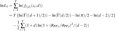
To estimate all the parameters together, we must maximize the log-likelihood of the sample of returns, which can be written
When we maximize  over all the parameters simultaneously, including the GARCH parameters implicit in
  , then we will typically get more precise parameter estimates compared with stepwise estimation of the GARCH parameters first and the distribution parameters second.
As a simple univariate example of the difference between quasi-maximum likelihood estimation (QMLE) and maximum likelihood estimate (MLE) consider the GARCH(1,1)- model with leverage. We have
6.2. An Easy Estimate of d
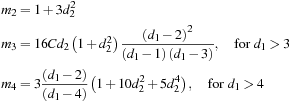
While the maximum likelihood estimation outlined here has nice properties, there is a very simple alternative estimation procedure available for the t distribution. If the conditional variance model has already been estimated, then we are only estimating one parameter, namely d. Because there is a simple closed-form relationship between d and the excess kurtosis, ζ2, this suggests first simply calculating ζ2 from the zt variable and then calculating d from
6.3. Calculating Value-at-Risk and Expected Shortfall
Once d is estimated, we can calculate the VaR for the portfolio return
Thus, we have
The formula for the expected shortfall is

6.4. QQ Plots
We can generalize the preceding QQ plot to assess the appropriateness of nonnormal distributions as well. In particular, we would like to assess if the returns standardized by the GARCH model conform to the  distribution.
However, the quantile of the standardized  distribution is usually not easily found in software packages, whereas the quantile from the conventional Student's
  distribution is. We therefore need the relationship

We are now ready to construct the QQ plot as
Figure 6.3 shows the QQ plot of the standardized returns from the GARCH- with leverage, estimated using QMLE. d is estimated to be 11.4. Notice that the t distribution fits the left tail better than the normal distribution, but this happens partly at the cost of fitting the right tail worse.
 |
| Figure 6.3 |
7. The Asymmetric t Distribution
The Student's t distribution can allow for kurtosis in the conditional distribution but not for skewness. It is possible, however, to develop a generalized, asymmetric version of the Student's t distribution. It is defined by pasting together two distributions at a point −A/B on the horizontal axis. The density function is defined by

 |
| Figure 6.4 |

Note from the formulas that although skewness is zero if d2 is zero, skewness and kurtosis are generally highly nonlinear functions of d1 and d2.
Consider again the two distributions in Figure 6.4. The red line corresponds to a skewness of +1 and an excess kurtosis of 2.6; the blue line corresponds to a skewness of −1 and an excess kurtosis of 2.6.
Skewness and kurtosis are both functions of d1 as well as d2. The upper panel of Figure 6.5 shows skewness plotted as a function of d2 on the horizontal axis. The blue line uses  (high kurtosis) and the red line uses
  (moderate kurtosis). The lower panel of Figure 6.5 shows kurtosis plotted as a function of d1 on the horizontal axis. The red line uses
  (no skewness) and the blue line uses
  (positive skewness). The asymmetric t distribution is capable of generating a wide range of skewness and kurtosis levels.

Notice that the symmetric standardized Student's t is a special case of the asymmetric t where  ,
,  , which implies A = 0 and B = 1, so we get
7.1. Estimation of d1 and d2
The parameters d1 and d2 in the asymmetric t distribution can be estimated via maximum likelihood as before. The only added complication is that the shape of the likelihood function on any given day will depend on the value of the shock zt. As before we can define the likelihood function for zt as

This estimation assumes that the conditional variance is estimated without error so that we can treat  as a regular data point. Alternatively joint estimation of the volatility and distribution parameters can be done using
We can also estimate d1 and d2 using sample estimates of skewness, ζ1, and kurtosis, ζ2. Unfortunately, the relationship between the parameters and the moments is nonlinear and so the equations
7.2. Calculating Value-at-Risk and Expected Shortfall
Once d1 and d2 are estimated, we can calculate the Value-at-Risk for the portfolio return

The expected shortfall can be computed as
7.3. QQ Plots
Armed with the earlier formula for the inverse cumulative density function (CDF) we can again construct the QQ plot as
Figure 6.6 shows the QQ plot for the asymmetric t distribution. Note that the asymmetric t distribution is able to fit the S&P 500 shocks quite well. Only the single largest negative shock seems to deviate substantially from the 45-degree line.
 |
| Figure 6.6 |
In conclusion, the asymmetric t distribution is somewhat cumbersome to estimate and implement but it is capable of fitting GARCH shocks from daily asset returns quite well.
The t distributions—and any other distribution—attempt to fit the entire range of outcomes using all the data available. Consequently, the estimated parameters in the distribution (for example d1 and d2) may be influenced excessively by data values close to zero, of which we observe many but of which risk managers care little about. We therefore now turn to an alternative approach that only makes use of the extreme return observations that of course contain crucial information for risk management.
8. Extreme Value Theory (EVT)
Typically, the biggest risks to a portfolio is the sudden occurrence of a single large negative return. Having explicit knowledge of the probabilities of such extremes is, therefore, at the essence of financial risk management. Consequently, risk managers ought to focus on modeling the tails of the returns distribution. Fortunately, a branch of statistics is devoted exactly to the modeling of such extreme values.
The central result in extreme value theory states that the extreme tail of a wide range of distributions can approximately be described by a relatively simple distribution, the so-called Generalized Pareto Distribution (GPD).
Virtually all results in extreme value theory (EVT) assume that returns are i.i.d. and therefore are not very useful unless modified to the asset return environment. Asset returns appear to approach normality at long horizons, thus EVT is more important at short horizons, such as daily. Unfortunately, the i.i.d. assumption is the least appropriate at short horizons due to the time-varying variance patterns. Therefore we need to get rid of the variance dynamics before applying EVT. Consider again, therefore, the standardized portfolio returns
Fortunately, it is typically reasonable to assume that these standardized returns are i.i.d. Thus, we will proceed to apply EVT to the standardized returns and then combine EVT with the variance models estimated in Chapter 4 and Chapter 5 in order to calculate VaR s.
8.1. The Distribution of Extremes
Consider the entire distribution of the shocks, zt, as illustrated for example by the histogram in Figure 6.1. EVT is concerned only with the tail of the distribution and we first have to decide what we mean by the tail. To this end define a threshold value u on the horizontal axis of the histogram. The threshold could for example be set to 0.02 in the top panel of Figure 6.1.
The key result in extreme value theory states that as you let the threshold u go to infinity, in almost any distribution you can think of, the distribution of observations beyond the threshold (call them y) converge to the Generalized Pareto Distribution,  , where
Standard distributions that are covered by the EVT result include those that are heavy tailed, for example the Student's t(d) distribution, where the tail-index parameter, ξ, is positive. This is, of course, the case of most interest in financial risk management, where returns tend to have fat tails.
The normal distribution is also covered. We noted earlier that a key difference between the Student's t(d) distribution and the normal distribution is that the former has power tails and the latter has exponential tails. Thus, for the normal distribution we have that the tail parameter, ξ, equals zero.
Finally, thin-tailed distributions are covered when the tail parameter ξ < 0, but they are not relevant for risk management and so we will not consider that case here.
8.2. Estimating the Tail Index Parameter, ξ
We could use MLE to estimate the GPD distribution defined earlier. However, if we are willing to assume that the tail parameter, ξ, is strictly positive, as is typically the case in risk management, then a very easy estimator exists, namely the so-called Hill estimator. The idea behind the Hill estimator is to approximate the GPD distribution by
We are now ready to construct the likelihood function for all observations yi larger than the threshold, u, as
Notice that our estimates are available in closed form—they do not require numerical optimization. They are, therefore, extremely easy to calculate.
So far we have implicitly referred to extreme returns as being large gains. Of course, as risk managers we are more interested in extreme negative returns corresponding to large losses. To this end, we simply do the EVT analysis on the negative of returns instead of returns themselves.
8.3. Choosing the Threshold, u
Until now, we have focused on the benefits of the EVT methodology, such as the explicit focus on the tails, and the ability to study each tail separately, thereby avoiding unwarranted symmetry assumptions. The EVT methodology does have an Achilles heel however, namely the choice of threshold, u. When choosing u we must balance two evils: bias and variance. If u is set too large, then only very few observations are left in the tail and the estimate of the tail parameter, ξ, will be very noisy. If on the other hand u is set too small, then the EVT theory may not hold, meaning that the data to the right of the threshold does not conform sufficiently well to the Generalized Pareto Distribution to generate unbiased estimates of ξ.
Simulation studies have shown that in typical data sets with daily asset returns, a good rule of thumb is to set the threshold so as to keep the largest 50 observations for estimating ξ; that is, we set Tu = 50. Visually gauging the QQ plot can provide useful guidance as well. Only those observations in the tail that are clearly deviating from the 45-degree line indicating the normal distribution should be used in the estimation of the tail index parameter, ξ.
8.4. Constructing the QQ Plot from EVT
We next want to show the QQ plot of the large losses using the EVT distribution. Define y to be a standardized loss; that is,
Next, we need to compute the inverse cumulative distribution function, which gives us the quantiles. Recall the EVT cumulative density function from before:
We are now ready to construct the QQ plot from EVT using the relationship
Figure 6.7 shows the QQ plots of the EVT tails for large losses from the standardized S&P 500 returns. For this data, ξ is estimated to be 0.22.

8.5. Calculating VaR and ES from the EVT Quantile
We are, of course, ultimately interested not in QQ plots but rather in portfolio risk measures such as Value-at-Risk. Using again the loss quantile  defined earlier by
The reason for using the (1 − p)th quantile from the EVT loss distribution in the VaR with coverage rate p is that the quantile such that  of losses are smaller than it is the same as minus the quantile such that
  of returns are smaller than it.
We usually calculate the VaR taking  to be the pth quantile from the standardized return so that
The expected shortfall can be computed using
In general, the ratio of ES to VaR for fat-tailed distribution will be higher than that of the normal. When using the Hill approximation of the EVT tail the previous formulas for VaR and ES show that we have a particularly simple relationship, namely
In Figure 6.8 we plot the tail shape of a normal distribution (the blue line) and EVT distribution (red line) where ξ = 0.5. The plot has been constructed so that the 1% VaR is 2.33 in both distributions. The probability mass under the two curves is therefore 1% in both cases. Note however, that the risk profile is very different. The normal distribution has a tail that goes to a virtual zero very quickly as the losses get extreme. The EVT distribution on the other hand implies a nontrivial probability of getting losses in excess of five standard deviations.
 |
| Figure 6.8 |
The preceding formula shows that when ξ = 0.5 then the ES to VaR ratio is 2. Thus even though the 1% VaR is the same in the two distributions by construction, the ES measure reveals the differences in the risk profiles of the two distributions, which arises from one being fat-tailed. The VaR does not reveal this difference unless the VaR is reported for several extreme coverage probabilities, p.
9. Summary
Time-varying variance models help explain nonnormal features of financial returns data. However, the distribution of returns standardized by a dynamic variance tends to be fat-tailed and may be skewed. This chapter has considered methods for modeling the nonnormality of portfolio returns by building on the variance and correlation models established in earlier chapters and using the same maximum likelihood estimation techniques.
We have introduced a graphical tool for visualizing nonnormality in the data, the so-called QQ plot. This tool was used to assess the appropriateness of alternative distributions.
Several alternative approaches were considered for capturing nonnormality in the portfolio risk distribution.
• The Filtered Historical Simulation approach, which uses the empirical distribution of the GARCH shocks and avoids making specific distribution choices
• The Cornish-Fisher approximation to the shock distribution, which allows for skewness and kurtosis using the sample moments that are easily estimated
• The standardized t distribution, which allows for fatter tails than the normal, but assumes that the distribution is symmetric around zero
• The asymmetric t distribution, which is more complex but allows for skewness as well as kurtosis
• Extreme value theory, which models the tail of the distribution directly using only extreme shocks in the sample
This chapter has focused on one-day-ahead distribution modeling. The multiday distribution requires Monte Carlo simulation, which will be covered in Chapter 8.
We end this chapter by stressing that in Part II of the book we have analyzed the conditional distribution of the aggregate portfolio return only. Thus, the distribution is dependent on the particular set of current portfolio weights, and the distribution must be reestimated when the weights change. Part III of the book presents multivariate risk models where portfolio weights can be rebalanced without requiring reestimation of the model.
Appendix A. ES for the Symmetric and Asymmetric t Distributions
In this appendix we derive the expected shortfall (ES) measure for the asymmetric t distribution. The ES for the symmetric case will be given as a special case at the end.
We want to compute  . Let us assume for simplicity that p is such that
  , then


Therefore,

In the symmetric case we have d1 = d, d2 = 0, A = 0, and B = 1 and so we get
Appendix B. Cornish-Fisher ES
The Cornish-Fisher approach assumes an approximate distribution of the form


Appendix C. Extreme Value Theory ES
Expected shortfall in the Hill approximation to EVT can be derived as

Further Resources
Details on the asymmetric t distribution considered here can be found in Hansen (1994), Fernandez and Steel (1998) and Jondeau and Rockinger (2003). Hansen (1994) and Jondeau and Rockinger (2003) also discuss time-varying skewness and kurtosis models. The GARCH- model was introduced by Bollerslev (1987).
Applications of extreme value theory to financial risk management is discussed in McNeil (1999). The choice of threshold value in the GARCH-EVT model is discussed in McNeil and Frey (2000). Huisman et al. (2001) explore improvements to the simple Hill estimator considered here. McNeil (1997) and McNeil and Saladin (1997) discuss the use of QQ plots in deciding on the threshold parameter, u. Brooks et al. (2005) compare various EVT approaches.
Multivariate extensions to the univariate EVT analysis considered here can be found in Longin (2000), Longin and Solnik (2001) and Poon et al. (2003).
The expected shortfall measure for the Cornish-Fisher approximation is developed in Giamouridis (2006). In the spirit of the Cornish-Fisher approach, Jondeau and Rockinger (2001) develop a Gram-Charlier approach to return distribution modeling.
Many alternative conditional distribution approaches exist. Kuerster et al. (2006) perform a large-scale empirical study.
GARCH and RV models can also be combined with jump processes. See Maheu and McCurdy (2004), Ornthanalai (2010) and Christoffersen et al. (2010).
Artzner et al. (1999) define the concept of a coherent risk measure and showed that expected shortfall (ES) is coherent whereas VaR is not. Studying dynamic portfolio management based on ES and VaR, Basak and Shapiro (2001) found that when a large loss does occur, ES risk management leads to lower losses than VaR risk management. Cuoco et al. (2008) argued instead that VaR and ES risk management lead to equivalent results as long as the VaR and ES risk measures are recalculated often. Both Basak and Shapiro (2001) and Cuoco et al. (2008) assumed that returns are normally distributed. Chen (2008) and Taylor (2008) consider nonparametric ES methods.
For analyses of GARCH-based risk models more generally see Bali et al. (2008), Mancini and Trojani (2011) and Jalal and Rockinger (2008).
Artzner, P.; Delbaen, F.; Eber, J.; Heath, D., Coherent measures of risk, Math. Finance 9 (1999) 203–228.
Bali, T.; Mo, H.; Tang, Y., The role of autoregressive conditional skewness and kurtosis in the estimation of conditional VaR, J. Bank. Finance 32 (2008) 269–282.
Basak, S.; Shapiro, A., Value at risk based risk management: Optimal policies and asset prices, Rev. Financ. Stud. 14 (2001) 371–405.
Bollerslev, T., A conditionally heteroskedastic time series model for speculative prices and rates of return, Rev. Econ. Stat. 69 (1987) 542–547.
Brooks, C.; Clare, A.; Molle, J.D.; Persand, G., A comparison of extreme value theory approaches for determining value at risk, J. Empir. Finance 12 (2005) 339–352.
Chen, S.X., Nonparametric estimation of expected shortfall, J. Financ. Econom 6 (2008) 87–107.
Christoffersen, P.; Jacobs, K.; Ornthanalai, C., Exploring time-varying jump intensities: Evidence from S&P 500 returns and options, Available from: SSRN,http://ssrn.com/abstract=1101733 (2010).
Cuoco, D.; He, H.; Issaenko, S., Optimal dynamic trading strategies with risk limits, Oper. Res. 56 (2008) 358–368.
Fernandez, C.; Steel, M.F.J., On Bayesian modeling of fat tails and skewness, J Am. Stat. Assoc. 93 (1998) 359–371.
Giamouridis, D., Estimation risk in financial risk management: A correction, J. Risk 8 (2006) 121–125.
Hansen, B., Autoregressive conditional density estimation, Int. Econ. Rev. 35 (1994) 705–730.
Huisman, R.; Koedijk, K.; Kool, C.; Palm, F., Tail-index estimates in small samples, J. Bus. Econ. Stat. 19 (2001) 208–216.
Jalal, A.; Rockinger, M., Predicting tail-related risk measures: The consequences of using GARCH filters for Non-GARCH data, J. Empir. Finance 15 (2008) 868–877.
Jondeau, E.; Rockinger, M., Gram-Charlier densities, J. Econ. Dyn. Control 25 (2001) 1457–1483.
Jondeau, E.; Rockinger, M., Conditional volatility, skewness and kurtosis: Existence, persistence and comovements, J. Econ. Dyn. Control 27 (2003) 1699–1737.
Kuerster, K.; Mittnik, S.; Paolella, M., Value-at-Risk prediction: A comparison of alternative strategies, J. Financ. Econom. 4 (2006) 53–89.
Longin, F., From value at risk to stress testing: The extreme value approach, J. Bank. Finance 24 (2000) 1097–1130.
Longin, F.; Solnik, B., Extreme correlation of international equity markets, J. Finance 56 (2001) 649–676.
Maheu, J.; McCurdy, T., News arrival, jump dynamics and volatility components for individual stock returns, J. Finance 59 (2004) 755–794.
Mancini, L.; Trojani, F., Robust value at risk prediction, J. Financ. Econom. 9 (2011) 281–313.
McNeil, A., Estimating the tails of loss severity distributions using extreme value theory, ASTIN Bull. 27 (1997) 117–137.
McNeil, A., Extreme value theory for risk managers, In: Internal modelling and CAD II (1999) Risk Books, London, pp. 23–43.
McNeil, A.; Frey, R., Estimation of tail-related risk measures for heteroskedastic financial time series: An extreme value approach, J. Empir. Finance 7 (2000) 271–300.
McNeil, A.; Saladin, T., The peaks over thresholds method for estimating high quantiles of loss distributions, In: Proceedings of the 28th International ASTIN ColloquiumCairns, Australia. (1997), pp. 23–43.
Ornthanalai, C., A new class of asset pricing models with Lévy processes: Theory and applications, Available from: SSRN,http://ssrn.com/abstract=1267432 (2010).
Poon, S.-H.; Rockinger, M.; Tawn, J., Extreme-value dependence measures and finance applications, Stat. Sin. 13 (2003) 929–953.
Taylor, J.W., Using exponentially weighted quantile regression to estimate value at risk and expected shortfall, J. Financ. Econom. 6 (2008) 382–406.
1. Construct a QQ plot of the S&P 500 returns divided by the unconditional standard deviation. Use the normal distribution. Compare your result with the top panel of Figure 6.2. (Excel hint: Use the NORMSINV function to calculate the standard normal quantiles.)
2. Copy and paste the estimated NGARCH(1,1) volatilities from Chapter 4.
3. Standardize the returns using the volatilities from exercise 2. Construct a QQ plot for the standardized returns using the normal distribution. Compare your result with the bottom panel of Figure 6.2.
4. Using QMLE, estimate the NGARCH(1,1)- model. Fix the variance parameters at their values from exercise 3. Set the starting value of d equal to 10. (Excel hint: Use the GAMMALN function for the log-likelihood function of the standardized t(d) distribution.)
Construct a QQ plot for the standardized returns using the standardized t(d) distribution. Compare your result with Figure 6.3. (Excel hint: Excel contains a two-sided quantile from the t(d) distribution. To compute one-sided quantiles from the standardized t(d) distribution, we use the relationship
5. Estimate the EVT model on the standardized portfolio returns using the Hill estimator. Use the 50 largest losses to estimate EVT. Calculate the 0.01% standardized return quantile implied by each of the following models: normal, t(d), EVT, and Cornish-Fisher. Notice how different the 0.01% VaR s would be from these four models.
6. Construct the QQ plot using the EVT distribution for the 50 largest losses. Compare your result with Figure 6.7.
7. For each day in 2010, calculate the 1-day, 1% VaR s using the following methods: (a) RiskMetrics, that is, normal distribution with an exponential smoother on variance using the weight  ; (b) NGARCH(1,1)-
 with the parameters estimated in exercise 5; (c) Historical Simulation; and (d) Filtered Historical Simulation. Use a 251-day moving sample for Historical Simulation. Plot the VaR s.
8. Use the asymmetric t distribution to construct Figure 6.4.
9. Use the asymmetric t distribution to construct Figure 6.5.
The answers to these exercises can be found in the Chapter6 Results.xlsx file, which is available from the companion site.
For more information see the companion site at http://www.elsevierdirect.com/companions/9780123744487
..................Content has been hidden....................
You can't read the all page of ebook, please click here login for view all page.