
5. Volatility Modeling Using Intraday Data
This chapter explores the use of intraday prices for computing daily volatility and for forecasting future volatility. We first introduce the concept of realized variance (RV) and look at four stylized facts of RV. We then look at different ways to forecast realized variance, as well as different ways to estimate realized variance, and we briefly look at some of the challenges of working with large and messy intraday data sets. At the end of the chapter we consider range-based proxies of daily volatility and also volatility forecast evaluation using RV and range-based volatility. Range-based volatilities are much easier to construct than RVs but in highly liquid markets RV will be more precise.
Keywords: Realized volatility, range-based volatility, market microstructure noise, sampling frequency
1. Chapter Overview
The goal of this chapter is to harness the information in intraday prices for computing daily volatility. Consider first estimating the mean of returns using a long sample of daily observations:
Consider now instead estimating variance on a sample of daily returns. We have
Imagine now having price observations at the end of every hour instead of every day and imagine that the market for the asset at hand (for example an FX rate) is open 24 hours a day. Now we would have 24 ⋅ T observations to estimate σ2 and we would get a much more precise estimate than when using just the T daily returns.
The dramatic implication for risk management of this high-frequency sampling idea is that just as we can use 21 daily prices to estimate a monthly volatility we can also use 24 hourly observations to estimate a daily volatility. If we have observations every minute then an even more precise estimate of daily volatility can be had and we can virtually treat daily volatility as an observed variable.
This chapter explores in detail the use of intraday prices for computing daily volatility and for forecasting future volatility. We first introduce the key concept of realized variance (RV) and look at four stylized facts of RV. We then look at ways to forecast RV and ways to estimate RV, and we briefly look at some of the challenges of working with large and messy intraday data sets. Toward the end of the chapter we look at range-based proxies of daily volatility and also at volatility forecast evaluation using RV and range-based volatility. Range-based volatilities are much easier to construct than RVs but in highly liquid markets RV will be more precise.
2. Realized Variance: Four Stylized Facts
Assume for simplicity that we are monitoring an asset that trades 24 hours per day and that is extremely liquid so that bid-ask spreads are virtually zero and new information is reflected in the price immediately. More realistic situations will be treated later. In an extremely liquid market with rapidly changing prices observed every second we can comfortably construct a time grid, for example, of 1-minute prices from which we can compute 1-minute log returns.
Let m be the number of observations per day on an asset. If we have 24 hour trading and 1-minute observations, then m = 24 ⋅ 60 = 1,440. Let the jth observation on day t + 1 be denoted St+j/m. Then the closing price on day t + 1 is St+m/m = St+1, and the jth 1-minute return is
The top panel of Figure 5.1 shows the time series of daily realized S&P 500 variance computed from intraday squared returns. The bottom panel shows the daily close-to-close squared returns S&P 500 as well. Notice how much more jagged and noisy the squared returns in the bottom panel are compared with the realized variances in the top panel. Figure 5.1 illustrates the first stylized fact of RV: RVs are much more precise indicators of daily variance than are daily squared returns.
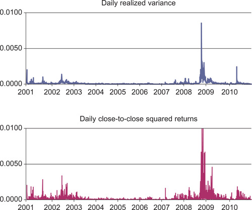 |
| Figure 5.1 |
The top panel of Figure 5.2 shows the autocorrelation function (ACF) of the S&P 500 RV series from Figure 5.1. The bottom panel shows the corresponding ACF computed from daily squared returns as in Chapter 4. Notice how much more striking the evidence of variance persistence is in the top panel. Figure 5.2 illustrates the second stylized fact of RV: RV is extremely persistent, which suggests that volatility may be forecastable at horizons beyond a few months as long as the information in intraday returns is used.

The top panel of Figure 5.3 shows a histogram of the RVs from Figure 5.1. The bottom panel of Figure 5.3 shows the histogram of the natural logarithm of RV. Figure 5.3 shows that the logarithm of RV is very close to normally distributed whereas the level of RV is strongly positively skewed with a long right tail.
 |
| Figure 5.3 |
Given that RV is a sum of squared returns it is not surprising that RV is not close to normally distributed but it is interesting and useful that a simple logarithmic transformation results in a distribution that is somewhat close to normal. The approximate log normal property of RV is the third stylized fact. We can write
The fourth stylized fact of RV is that daily returns divided by the square root of RV is very close to following an i.i.d. (independently and identically distributed) standard normal distribution. We can write
The fourth stylized fact suggests that if a good forecast of  , call it
  , can be made using information available at time t then a normal distribution assumption of
  will be a decent first modeling strategy. Approximately
Constructing a good forecast for  is the topic to which we now turn. When doing so we will need to keep in mind the four stylized facts of RV:
• RV is a more precise indicator of daily variance than is the daily squared return.
• RV has large positive autocorrelations for many lags.
• The log of RV is approximately normally distributed.
• The daily return divided by the square root of RV is close to i.i.d. standard normal.
3. Forecasting Realized Variance
Realized variances are very persistent and so the main task at hand is to consider forecasting models that allow for current RV to matter for future RV.
3.1. Simple ARMA Models of Realized Variance
In Chapter 3 we introduced the AR(1) model as a simple way to allow for persistence in a time series. If we treat the estimated  as an observed time series, then we can assume the AR(1) forecasting model
Given that we observed in Figure 5.3 that the log of RV is close to normally distributed we may be better off modeling the RV in logs rather than levels. We can therefore assume
Because we have estimated it from intraday squared returns, the  series is not truly an observed time series but it can be viewed as the true RV observed with a measurement error. If the true RV is AR(1) but we observed true RV plus an i.i.d. measurement error then an ARMA(1,1) model is likely to provide a good fit to the observed RV. We can write
Notice that these simple models are specified in logarithms, while for risk management purposes we are ultimately interested in forecasting the level of variance. As the exponential function is not linear, we have in the log RV model that
From the assumption of normality of the error term we can use the result
In the AR(1) model the forecast for tomorrow is

More sophisticated models such as long-memory (or fractionally integrated) ARMA models can be used to model realized variance. These models may yield better longer horizon variance forecasts than the short-memory ARMA models considered here. As a simple but powerful way to allow for more persistence in the variance forecasting model we next consider the so-called heterogeneous AR models.
3.2. Heterogeneous Autoregressions (HAR)
The question arises whether we can parsimoniously (that is with only few parameters) and easily (that is using OLS) model the apparent long-memory features of realized volatility. The mixed-frequency or heterogeneous autoregression model (HAR) we now consider provides an affirmative answer to this question. Define the h-day RV from the 1-day RV as follows:
Given that economic activity is organized in days, weeks, and months, it is natural to consider forecasting tomorrow's RV using daily, weekly, and monthly RV defined by the simple moving averages

The HAR will be able to capture long-memory-like dynamics because 21 lags of daily RV matter in this model. The model is parsimonious because the 21 lags of daily RV do not have 21 different autoregressive coefficients: The coefficients are restricted to be  on today's RV,
  on the past four days of RV, and
  on the RVs for days t − 20 through t − 5.
Given the log normal property of RV we can also consider HAR models of the log transformation of RV:
The advantage of this log specification is again that the parameters will be estimated more precisely when using OLS. Remember though that forecasting involves undoing the log transformation so that
 |
| Figure 5.4 |
In Chapter 4 we saw the importance of including a leverage effect in the GARCH model capturing that volatility rises more on a large positive return than on a large negative return. The HAR model can capture this by simply including the return on the right-hand side. In the daily log HAR we can write
The stylized facts of RV suggested that we can assume that
3.3. Combining GARCH and RV
So far in Chapters 4 and 5 we have considered two seemingly very different approaches to volatility modeling: In Chapter 4 GARCH models were estimated on daily returns, and in Chapter 5 time-series models of daily RV have been constructed from intraday returns. We can instead try to incorporate the rich information in RV into a GARCH modeling framework. Consider the basic GARCH model from Chapter 4:
A shortcoming of the GARCH-X approach is that a model for RV is not specified. This means that we cannot use the model to forecast volatility beyond one day ahead.
The more general so-called Realized GARCH model is defined by

4. Realized Variance Construction
So far we have assumed that a grid of highly liquid 1-minute prices are available so that the corresponding 1-minute log returns are informative about the true volatility of the asset price. However, once various forms of illiquidity in the asset price are considered it becomes clear that we need to be much more clever about constructing the RVs from the intraday returns. This section is devoted to the construction of unbiased daily RVs from intraday returns under realistic assumptions about market liquidity.
4.1. The All RV Estimator
Remember that in the ideal but unfortunately unrealistic case with ultra-high liquidity we have m = 24 ⋅ 60 observations available within a day, and we can calculate an estimate of the daily variance from the intraday squared returns simply as
Figure 5.5 uses simulated data to illustrate one of the problems caused by illiquidity when estimating asset price volatility. We assume the fundamental (but unobserved) asset price, SFund, follows the simple random walk process with constant variance
 |
| Figure 5.5 |
The challenge is that we observe  but want to estimate σ2, which is the variance of the unobserved
  . Figure 5.5 shows that the observed intraday price can be very noisy compared with the smooth fundamental but unobserved price. The bid-ask spread adds a layer of noise on top of the fundamental price. If we compute
  from the high-frequency
  then we will get an estimate of σ2 that is higher than the true value because of the inclusion of the bid-ask volatility in the estimate.
4.2. The Sparse RV Estimator
The perhaps simplest way to address the problem shown in Figure 5.5 is to construct a grid of intraday prices and returns that are sampled less frequently than the 1-minute assumed earlier. Instead of a 1-minute grid we could use an s-minute grid (where s ≥ 1) so that our new RV estimator would be
Of course the important question is how to choose the parameter s? Should s be 5 minutes, 10 minutes, 30 minutes, or an even lower frequency? The larger the s the less likely we are to get a biased estimate of volatility, but the larger the s the fewer observations we are using and so the more noisy our estimate will be. We are faced with a typical variance-bias trade-off.
The choice of s clearly depends on the specific asset. For very liquid assets we should use an s close to 1 and for illiquid assets s should be much larger. If liquidity effects manifest themselves as a bias in the estimated RVs when using a high sampling frequency then that bias should disappear when the sampling frequency is lowered; that is, when s is increased.
The so-called volatility signature plots provide a convenient graphical tool for choosing s: First compute  for values of s going from 1 to 120 minutes. Second, scatter plot the average RV across days on the vertical axis against s on the horizontal axis. Third, look for the smallest s such that the average RV does not change much for values of s larger than this number.
In markets with wide bid–ask spreads the average RV in the volatility signature plot will be downward sloping for small s but for larger s the average RV will stabilize at the true long run volatility level. We want to choose the smallest s for which the average RV is stable. This will avoid bias and minimize variance.
In markets where trading is thin, new information is only slowly incorporated into the price, and intraday returns will have positive autocorrelation resulting in an upward sloping volatility signature plot. In this case, the rule of thumb for computing RV is again to choose the smallest s for which the average RV has stabilized.
4.3. The Average RV Estimator
Choosing a lower (sparse) frequency for the grid of intraday prices can solve the bias problem arising from illiquidity but it will also increase the noise of the RV estimator. When we are using sparse sampling we are essentially throwing away information, which seems wasteful. It turns out that there is an amazingly simple way to lower the noise of the Sparse RV estimator without increasing the bias.
Let us say that we have used the volatility signature plot to chose s = 15 in the Sparse RV so that we are using a 15-minute grid for prices and squared returns to compute RV. Note that if we have the original 1-minute grid (of less liquid prices) then we can actually compute 15 different (but overlapping) Sparse RV estimators. The first Sparse RV will use a 15-minute grid starting with the 15-minute return at midnight, call it  ; the second will also use a 15-minute grid but this one will be starting one minute past midnight, call it
  , and so on until the 15th Sparse RV, which uses a 15-minute grid starting at 14 minutes past midnight, call it
  . We are thus using the fine 1-minute grid to compute 15 Sparse RVs at the 15-minute frequency.
We have now used all the information on the 1-minute grid but we have used it to compute 15 different RV estimates, each based on 15-minute returns, and none of which are materially affected by illiquidity bias. By simply averaging the 15 sparse RVs we get the so-called Average RV estimator
4.4. RV Estimators with Autocovariance Adjustments
Instead of using sparse sampling to avoid RV bias we can try to model and then correct for the autocorrelations in intraday returns that are driving the volatility bias.
Assume that the fundamental log price is observed with an additive i.i.d. error term, u, caused by illiquidity so that
In this case the observed log return will equal the true fundamental returns plus an MA(1) error:
The All RV in this case is defined by
If we are fairly confident that the measurement error is of the MA(1) form then we know (see Chapter 3) that only the first-order autocorrelations are nonzero and we can therefore easily correct the RV estimator as follows:
Positive autocorrelation caused by slowly changing prices would be at least partly captured by the first-order autocorrelation as well. It would be positive in this case and we would have
Much more general estimators have been developed to correct for more complex autocorrelation patterns in intraday returns. References to this work will be listed at the end of the chapter.
5. Data Issues
So far we have assumed the availability of a 1-minute grid of prices in a 24-hour market. But in reality several challenges arise. First, prices and quotes arrive randomly in time and not on a neat, evenly spaced grid. Second, markets are typically not open 24 hours per day. Third, intraday data sets are large and messy and often include price and quote errors that must be flagged and removed before estimating volatility. We deal with these three issues in turn as we continue.
5.1. Dealing with Irregularly Spaced Intraday Prices
The preceding discussion has assumed that a sample of regularly spaced 1-minute intraday prices are available. In practice, transaction prices or quotes arrive in random ticks over time and the evenly spaced price grid must be constructed from the raw ticks.
The first and simplest solution is to use the last tick prior to a grid point as the price observation for that grid point. This way the last observed tick price in an interval is effectively moved forward in time to the next grid point. Specifically, assume we have N observed tick prices during day t + 1 but that these are observed at irregular times  ,
,  ,…,
,…, Consider now the j th point on the evenly spaced grid of m points for day t + 1, which we have called
  . Grid point
  will fall between two adjacent randomly spaced ticks, say the i th and the
  th; that is, we have
  and in this case we choose the
  price to be
The second and slightly less simple solution uses a linear interpolation between St(i) and St(i + 1) so what we have
While the linear interpolation method makes some intuitive sense it has poor limiting properties: The smoothing implicit in the linear interpolation makes the estimated RV go to zero in the limit. Therefore, using the most recent tick on each grid point has become standard practice.
5.2. Choosing the Frequency of the Fine Grid of Prices
Notice that we still have to choose the frequency of the fine grid. We have used 1-minute as an example but this number is clearly also asset dependent. An asset with N = 2,000 new quotes on average per day should have a finer grid than an asset with N = 50 new quotes on average per day.
We ought to have at least one quote per interval on the fine grid. So we should definitely have that m < N. However, the distribution of quotes is typically very uneven throughout the day and so setting m close to N is likely to yield many intervals without new quotes. We can capture the distribution of quotes across time on each day by computing the standard deviation of  across i on each day.
The total number of new quotes, N, will differ across days and so will the standard deviation of the quote time intervals. Looking at the descriptive statistics of N and the standard deviation of quote time intervals across days is likely to yield useful guidance on the choice of m.
5.3. Dealing with Data Gaps from Overnight Market Closures
In risk management we are typically interested in the volatility of 24-hour returns (the return from the close of day t to the close on day t + 1) even if the market is only open, say, 8 hours per day. In Chapter 4 we estimated GARCH models on daily returns from closing prices. The volatility forecasts from GARCH are therefore by construction 24-hour return volatilities.
If we care about 24-hour return volatility and we only have intraday returns from market open to market close, then the RV measure computed on intraday returns, call it  , must be adjusted for the return in the overnight gap from close on day t to open on day t + 1. There are three ways to make this adjustment.
First, we can simply scale up the market-open RV measure using the unconditional variance estimated from daily squared returns:
Second, we can add to  the squared return constructed from the close on day t to the open on day t + 1:
Notice that this sum puts equal weight on the two terms and thus a relatively high weight on the close-to-open gap for which little information is available. Note also that  is simply the daily price observation that we denoted St in the previous chapters.
A third, but more cumbersome approach is to find optimal weights for the two terms. This can be done by minimizing the variance of the  estimator subject to having a bias of zero.
When computing optimal weights typically a much larger weight is found for  than for
  . This suggests that scaling up the
  may be the better of the two first approaches to correcting for the overnight gap.
5.4. Alternative RV Estimators Using Tick-by-Tick Data
There is an alternative set of RV estimators that avoid the construction of a time grid altogether and instead work directly with the irregularly spaced tick-by-tick data. Let the i th tick return on day t + 1 be defined by
Notice that tick-time sampling avoids sampling the same observation multiple times, which could happen on a fixed grid if the grid is too fine compared with the number of available intraday prices.
The preceding simple tick-based RV estimator can be extended by allowing for autocorrelation in the tick-time returns.
The optimality of grid-based versus tick-based RV estimators depends on the structure of the market for the asset and on its liquidity. The majority of academic research relies on grid-based RV estimators.
5.5. Price and Quote Data Errors
The construction of the intraday price grid is perhaps the most challenging task when estimating and forecasting volatility using realized variance. The raw intraday price data contains observations randomly spaced in time and the sheer volume of data can be enormous when investigating many assets over long time periods.
The construction of the grid of prices is complicated by the presence of data errors. A data error is broadly defined as a quoted price that does not conform to the real situation of the market. Price data errors could take several forms:
• Decimal errors; for example, when a bid price changes from 1.598 to 1.603 but a 1.503 is reported instead of 1.603.
• Test quotes: These are quotes sent by a contributor at early mornings or at other inactive times to test the system. They can be difficult to catch since the prices may look plausible.
• Repeated ticks: These are sent automatically by contributors. If sent frequently, then they can obstruct the filtering of a few informative quotes sent by other contributors.
• Tick copying: Contributors automatically copy and resend quotes of other contributors to show a strong presence in the market. Sometimes random error is added so as to hide the copying aspect.
• Scaling problems: The scale of the price of an asset may differ by contributor and it may change over time without notice.
Given the size of intraday data sets it is impossible to manually check for errors. Automated filters must be developed to catch errors of the type just listed. The challenges of filtering intraday data has created a new business for data vendors. OlsenData.com and TickData.com are examples of data vendors that sell filtered as well as raw intraday data.
6. Range-Based Volatility Modeling
The construction of daily realized volatilities relies on the availability of intraday prices on relatively liquid assets. For markets that are not liquid, or for assets where historical information on intraday prices is not available the intraday range presents a convenient alternative.
The intraday price range is based on the intraday high and intraday low price. Casual browsing of the web (see for example finance.yahoo.com) reveals that these intraday high and low prices are easily available for many assets far back in time. Range-based variance proxies are therefore easily computed.
6.1. Range-Based Proxies for Volatility
Let us define the range of the log prices to be
We can show that if the log return on the asset is normally distributed with zero mean and variance, σ2, then the expected value of the squared range is
The range-based estimate of unconditional variance suggests that a range proxy for the daily variance can be constructed as
The top panel of Figure 5.6 plots RPt for the S&P 500 data.
 |
| Figure 5.6 |
Notice how much less noisy the range is than the daily squared returns that are shown in the bottom panel.
Figure 5.7 shows the autocorrelation of RPt in the top panel. The first-order autocorrelation in the range-based variance proxy is around 0.60 (top panel) whereas it is only half of that in the squared-return proxy (bottom panel). Furthermore, the range-based autocorrelations are much smoother and thus give a much more reliable picture of the persistence in variance than do the squared returns in the bottom panel.

This range-based volatility proxy does not make use of the daily open and close prices, which are also easily available and which also contain information about the 24-hour volatility. Assuming again that the asset log returns are normally distributed with zero mean and variance, σ2, then a more accurate range-based proxy can be derived as
In the more general case where the mean return is not assumed to be zero the following range-based volatility proxy is available:
6.2. Forecasting Volatility Using the Range
Perhaps the simplest approach to using RPt in a forecasting model is to use it in place of RV in the earlier AR and HAR models. Although RPt may be more noisy than RV, the HAR approach should yield good forecasting results because the HAR model structure imposes a lot of smoothing.
The strong persistence of the range as well as the log normal property suggest a log HAR model of the form
Finally, a Realized-GARCH style model (let us call it Range-GARCH) can be defined via

The Range-GARCH model can be estimated using bivariate maximum likelihood techniques using historical data on return, Rt, and on the range proxy, RPt.
ES and VaR can be constructed in the RP-based models in the same way as in the RV-based models by assuming that zt + 1 is i.i.d. normal where  in the GARCH-style models or
  in the HAR model.
6.3. Range-Based versus Realized Variance
There is convincing empirical evidence that for very liquid securities the RV modeling approach is useful for risk management purposes. The intuition is that using the intraday returns gives a very reliable estimate of today's variance, which in turn helps forecast tomorrow's variance. In standard GARCH models on the other hand, today's variance is implicitly calculated using exponentially declining weights on many past daily squared returns, where the exact weighting scheme depends on the estimated parameters. Thus the GARCH estimate of today's variance is heavily model dependent, whereas the realized variance for today is calculated exclusively from today's squared intraday returns. When forecasting the future, knowing where you are today is key. Unfortunately in variance forecasting, knowing where you are today is not a trivial matter since variance is not directly observable.
While the realized variance approach has clear advantages it also has certain shortcomings. First of all it clearly requires high-quality intraday returns to be feasible. Second, it is very easy to calculate daily realized volatilities from 5-minute returns, but it is not at all a trivial matter to construct at 10-year data set of 5-minute returns.
Figure 5.5 illustrates that the observed intraday price can be quite noisy compared with the fundamental but unobserved price. Therefore, realized variance measures based on intraday returns can be noisy as well. This is especially true for securities with wide bid–ask spreads and infrequent trading. Notice on the other hand that the range-based variance measure discussed earlier is relatively immune to the market microstructure noise. The true maximum can easily be calculated as the observed maximum less one half of the bid–ask spread, and the true minimum as the observed minimum plus one half of the bid–ask price. The range-based variance measure thus has clear advantages in less liquid markets.
In the absence of trading imperfections, however, range-based variance proxies can be shown to be only about as useful as 4-hour intraday returns. Furthermore, as we shall see in Chapter 7, the idea of realized variance extends directly to realized covariance and correlation, whereas the range-based covariance and correlation measures are less obvious.
7. GARCH Variance Forecast Evaluation Revisited
In the previous chapter we briefly introduced regressions using daily squared returns to evaluate the GARCH model forecasts. But we quickly argued that daily returns are too noisy to proxy for observed daily variance. In this chapter we have developed more informative proxies based on RV and RP and they should clearly be useful for variance forecast evaluation.
The realized variance measure can be used instead of the squared return for evaluating the forecasts from variance models. If only squared returns are available then we can run the regression
If we have RV-based estimates available then we would instead run the regression
The range-based proxy could of course also be used instead of the squared return for evaluating the forecasts from variance models. Thus we could run the regression
Using  on the left-hand side of these regressions is likely to yield the finding that the volatility forecast is poor. The fit of the regression will be low but notice that this does not necessarily mean that the volatility forecast is poor. It could also mean that the volatility proxy is poor. If regressions using
  or
or  yield a much better fit than the regression using
  then the volatility forecast is much better than suggested by the noisy squared-return proxy.
8. Summary
Realized volatility and range-based volatility are likely to be much more informative about daily volatility than is the daily squared return. This fact has important implications for the evaluation of volatility forecasts but it has even more important implications for volatility forecast construction. If intraday information is available then it should be used to construct more accurate volatility forecasts than those that can be constructed from daily returns alone. This chapter has introduced a number of practical approaches to volatility forecasting using intraday information.
Further Resources
The classic references on realized volatility include Andersen et al., 2001 and Andersen et al., 2003 and Barndorff-Nielsen and Shephard (2002). See the survey in Andersen et al. (2010) for a thorough literature review.
The HAR model for RV was developed in Corsi (2009) and has been used in Andersen et al. (2007b) among others. Engle (2002) suggested RV in the GARCH-X model and the Realized GARCH model was developed in Hansen et al. (2011). See also the HEAVY model in Shephard and Sheppard (2010).
The crucial impact on RV of liquidity and market microstructure effects more generally has been investigated in Andersen et al. (2011), Bandi and Russell (2006) and Ait-Sahalia and Mancini (2008).
The choice of sampling frequency has been analyzed by Ait-Sahalia et al. (2005) and Bandi and Russell (2008). The volatility signature plot was suggested in Andersen et al. (1999). The Average RV estimator is discussed in Zhang et al. (2005). The RV estimates corrected for return autocorrelations were developed by Zhou (1996), Barndorff-Nielsen et al. (2008) and Hansen and Lunde (2006).
The use of RV in volatility forecast evaluation was pioneered by Andersen and Bollerslev (1998). See also Andersen et al., 2004 and Andersen et al., 2005 and Patton (2011).
The use of RV in risk management is discussed in Andersen et al. (2007a) and the use of RV in portfolio allocation is developed in Bandi et al. (2008) and Fleming et al. (2003).
For forecasting applications of RV see Martens (2002), Thomakos and Wang (2003), Pong et al. (2004), Koopman et al. (2005) and Maheu and McCurdy (2011).
For treating overnight gaps see Hansen and Lunde (2005) and for data issues in RV construction see Brownlees and Gallo (2006), Muller (2001) and Dacorogna et al. (2001).
Range-based estimates variance models are introduced in Parkinson (1980) and Garman and Klass (1980) and more recent contributions include Rogers and Satchell (1991) and Yang and Zhang (2000). Range-based models of dynamic variance are developed in Azalideh et al. (2002), Brandt and Jones (2006) and Chou (2005) and they are surveyed in Chou et al. (2009). Brandt and Jones (2006) use the range rather than the squared return as the fundamental innovation in an EGARCH model and find that the range improves the model's variance forecasts significantly.
Ait-Sahalia, Y.; Mancini, L., Out of sample forecasts of quadratic variation, J. Econom. 147 (2008) 17–33.
Ait-Sahalia, Y.; Mykland, P.A.; Zhang, L., How often to sample a continuous-time process in the presence of market microstructure noise, Rev. Financ. Stud. 18 (2005) 351–416.
Andersen, T.G.; Bollerslev, T., Answering the skeptics: Yes, standard volatility models do provide accurate forecasts, Int. Econ. Rev. 39 (1998) 885–905.
Andersen, T.; Bollerslev, T.; Christoffersen, P.; Diebold, F.X., Practical volatility and correlation modeling for financial market risk management, In: (Editors: Carey, M.; Stulz, R.) The NBER Volume on Risks of Financial Institutions (2007) University of Chicago Press, Chicago, IL.
Andersen, T.G.; Bollerslev, T.; Diebold, F.X., Roughing it up: Including jump components in the measurement, modeling and forecasting of return volatility, Rev. Econ. Stat. 89 (2007) 701–720.
Andersen, T.G.; Bollerslev, T.; Diebold, F.X., Parametric and nonparametric measurements of volatility, In: (Editors: Ait-Sahalia, Y.; Hansen, L.P.) Handbook of Financial Econometrics (2010) North-Holland, Amsterdam, The Netherlands, pp. 67–138.
Andersen, T.G.; Bollerslev, T.; Diebold, F.X.; Labys, P., (Understanding, optimizing, using and forecasting) Realized volatility and correlation, published in revised form as “Great Realizations, .” Risk March 2000 (1999) 105–108.
Andersen, T.G.; Bollerslev, T.; Diebold, F.X.; Labys, P., The distribution of exchange rate volatility, J. Am. Stat. Assoc. 96 (2001) 42–55.
Andersen, T.G.; Bollerslev, T.; Diebold, F.X.; Labys, P., Modeling and forecasting realized volatility, Econometrica 71 (2003) 579–625.
Andersen, T.G.; Bollerslev, T.; Meddahi, N., Analytic evaluation of volatility forecasts, Int. Econ. Rev. 45 (2004) 1079–1110.
Andersen, T.G.; Bollerslev, T.; Meddahi, N., Correcting the errors: Volatility forecast evaluation using high-frequency data and realized volatilities, Econometrica 73 (2005) 279–296.
Andersen, T.; Bollerslev, T.; Meddahi, N., Realized volatility forecasting and market microstructure noise, J. Econom. 160 (2011) 220–234.
Azalideh, S.; Brandt, M.; Diebold, F.X., Range-based estimation of stochastic volatility models, J. Finance 57 (2002) 1047–1091.
Bandi, F.; Russell, J., Separating microstructure noise from volatility, J. Financ. Econ. 79 (2006) 655–692.
Bandi, F.; Russell, J., Microstructure noise, realized volatility, and optimal sampling, Rev. Econ. Stud. 75 (2008) 339–369.
Bandi, F.; Russell, J.; Zhu, Y., Using high-frequency data in dynamic portfolio choice, Econom. Rev. 27 (2008) 163–198.
Barndorff-Nielsen, O.E.; Hansen, P.; Lunde, A.; Shephard, N., Designing realised kernels to measure the ex-post variation of equity prices in the presence of noise, Econometrica 76 (2008) 1481–1536.
Barndorff-Nielsen, O.E.; Shephard, N., Econometric analysis of realised volatility and its use in estimating stochastic volatility models, J. Royal Stat. Soc. B 64 (2002) 253–280.
Brandt, M.; Jones, C., Volatility forecasting with range-based EGARCH models, J. Bus. Econ. Stat. 24 (2006) 470–486.
Brownlees, C.; Gallo, G.M., Financial econometric analysis at ultra-high frequency: Data handling concerns, Comput. Stat. Data Anal. 51 (2006) 2232–2245.
Chou, R., Forecasting financial volatilities with extreme values: The conditional autoregressive range, J. Money Credit Bank. 37 (2005); 561–82.
Chou, R.; Chou, H.-C.; Liu, N., Range volatility models and their applications in finance, In: (Editors: Lee, C.-F.; Lee, J.) Handbook of Quantitative Finance and Risk Management (2009) Springer, New York, NY, pp. 1273–1281.
Corsi, F., A simple approximate long memory model of realized volatility, J. Financ. Econom. 7 (2009) 174–196.
Dacorogna, M.; Gencay, R.; Muller, U.; Olsen, R.; Pictet, O., An Introduction to High-Frequency Finance. (2001) Academic Press, San Diego, CA.
Engle, R., New frontiers in ARCH models, J. Appl. Econom. 17 (2002) 425–446.
Fleming, J.; Kirby, C.; Oestdiek, B., The economic value of volatility timing using ‘realized’ volatility, with Jeff Fleming and Chris Kirby, J. Financ. Econ. 67 (2003) 473–509.
Garman, M.; Klass, M., On the estimation of securities price volatilities from historical data, J. Bus. 53 (1980) 67–78.
Hansen, P.; Huang, Z.; Shek, H., Realized GARCH: A joint model for returns and realized measures of volatility, J. Appl. Econom. (2011); forthcoming.
Hansen, P.; Lunde, A., A realized variance for the whole day based on intermittent high-frequency data, J. Financ. Econom. 3 (2005) 525–554.
Hansen, P.; Lunde, A., Realized variance and market microstructure noise, J. Bus. Econ. Stat. 24 (2006) 127–161.
Koopman, S.J.; Jungbacker, B.; Hol, E., Forecasting daily variability of the S&P 100 stock index using historical, realized and implied volatility measures, J. Empir. Finance 12 (2005) 445–475.
Maheu, J.; McCurdy, T., Do high-frequency measures of volatility improve forecasts of return distributions?J. Econom. 160 (2011) 69–76.
Martens, M., Measuring and forecasting S&P 500 index futures volatility using high-frequency data, J. Futures Mark. 22 (2002) 497–518.
Muller, U., The Olsen filter for data in finance. (2001) Working paper, O&A Research Group; Available from: http://www.olsendata.com.
Parkinson, M., The extreme value method for estimating the variance of the rate of return, J. Bus. 53 (1980) 61–65.
Patton, A., Volatility forecast comparison using imperfect volatility proxies, J. Econom. 160 (2011) 246–256.
Pong, S.; Shackleton, M.B.; Taylor, S.J.; Xu, X., Forecasting currency volatility: A comparison of implied volatilities and AR(FI)MA models, J. Bank. Finance 28 (2004) 2541–2563.
Rogers, L.; Satchell, S., Estimating variance from high, low and closing prices, Ann. Appl. Probab. 1 (1991) 504–512.
Shephard, N.; Sheppard, K., Realizing the future: Forecasting with high-frequency-based volatility (HEAVY) models, J. Appl. Econom. 25 (2010) 197–231.
Thomakos, D.D.; Wang, T., Realized volatility in the futures market, J. Empir. Finance 10 (2003) 321–353.
Yang, D.; Zhang, Q., Drift-independent volatility estimation based on high, low, open, and close prices, J. Bus. 73 (2000) 477–491.
Zhang, L.; Mykland, P.A.; Ait-Sahalia, Y., A tale of two time scales: Determining integrated volatility with noisy high-frequency data, J. Am. Stat. Assoc. 100 (2005) 1394–1411.
Zhou, B., High-frequency data and volatility in foreign exchange rates, J. Bus. Econ. Stat. 14 (1996) 45–52.
1. Run a regression of daily squared returns on the variance forecast from the GARCH model with a leverage term from Chapter 4. Include a constant term in the regression
2. Run a regression using RP instead of the squared returns as proxies for observed variance; that is, regress
3. Run a regression using RV instead of the squared returns as proxies for observed variance; that is, regress
4. Estimate a HAR model in logarithms on the RP data you constructed in exercise 2. Use the next day's RP on the left-hand side and use daily, weekly, and monthly regressors on the right-hand side. Compute the regression fit.
5. Estimate a HAR model in logarithms on the RV data. Use the next day's RV on the left-hand side and use daily, weekly, and monthly regressors on the right-hand side. Compare the regression fit from this equation with that from exercise 4.
The answers to these exercises can be found in the Chapter5 Results.xls file, which can be found on the companion site.
For more information see the companion site at http://www.elsevierdirect.com/companions/9780123744487
..................Content has been hidden....................
You can't read the all page of ebook, please click here login for view all page.