
12. Credit Risk Management
This chapter introduces credit risk, which can be defined as the risk of loss due to a counterparty's failure to honor an obligation. Default risk, which is a key element of credit risk, introduces an important source of nonnormality into the portfolio distribution. We first introduce the Merton model to help us understand default of a single counterparty. Default risk has an important effect on how corporate debt is priced, but default risk will also impact the equity price. We build on the single-firm Merton model to develop a factor model of credit portfolio risk. The portfolio model provides a framework for computing credit Value-at-Risk. Finally, the chapter introduces credit default swaps, which give a market-based view of default risk.
Keywords: Default, recovery, Merton model, Vasicek distribution, credit VaR, credit default swaps.
1. Chapter Overview
Credit risk can be defined as the risk of loss due to a counterparty's failure to honor an obligation in part or in full. Credit risk can take several forms. For banks credit risk arises fundamentally through its lending activities. Nonbank corporations that provide short-term credit to their debtors face credit risk as well. But credit risk can be important not only for banks and other credit providers; in certain cases it is important for investors as well.
Investors who hold a portfolio of corporate bonds or distressed equities need to get a handle on the default probability of the assets in their portfolio. Default risk, which is a key element of credit risk, introduces an important source of nonnormality into the portfolio in this case.
Credit risk can also arise in the form of counterparty default in a derivatives transaction. Figure 12.1 illustrates the counterparty risk exposure of a derivative contract. The horizontal axis shows the value of a hypothetical derivative contract in the absence of counterparty default risk. The derivative contract can have positive or negative value to us depending on the value of the asset underlying the derivative contract. The vertical axis shows our exposure to default of the derivative counterparty. When the derivative contract has positive value for us then counterparty risk is present. If the counterparty defaults then we might lose the entire value of the derivative and so the slope of the exposure is + 1 to the right of zero in Figure 12.1. When the derivative contract has negative value to us then the default of our counterparty will have no effect on us; we will owe the same amount regardless. The counterparty risk is zero in this case.
 |
| Figure 12.1 |
It is clear from Figure 12.1 that counterparty default risk has an option-like structure. Note that unlike in Chapter 10 and Chapter 11, Figure 12.1 has loss on the vertical axis instead of gain. Counterparty default risk can therefore be viewed as having sold a call option. Figure 12.1 ignores the fact that part of the value of the derivative position may be recovered in case of counterparty default. Partial recovery will be discussed later.
The chapter is structured as follows:
•Section 2 provides a few stylized facts on corporate defaults.
•Section 3 develops a model for understanding the effect on corporate debt and equity values of corporate default. Not surprisingly, default risk will have an important effect on how corporate debt (think a corporate bond) is priced, but default risk will also impact the equity price. The model will help us understand which factors drive corporate default risk.
•Section 5 discusses a range of further issues in credit risk including recovery rates, measuring credit quality through ratings, and measuring default risk using credit default swaps.
2. A Brief History of Corporate Defaults
Credit rating agencies such as Moody's and Standard & Poor's maintain databases of corporate defaults through time. In Moody's definition corporate default is triggered by one of three events: (1) a missed or delayed interest or principal payment, (2) a bankruptcy filing, or (3) a distressed exchange where old debt is exchanged for new debt that represents a smaller obligation for the borrower.
Table 12.1 shows some of the largest defaults in recent history. In terms of nominal size, the Lehman default in September 2008 clearly dominates. It is also interesting to note the apparent industry concentration of large defaults. The defaults in financial services companies is of course particularly concerning from the point of view of counterparty risk in derivatives transactions.
| Notes: The table shows the largest defaults (by default volume) of the firms rated by Moody's during the 1920 through 2008 period. The data is from Moody's (2011). | ||||
| Company | Default Volume ($ mill) | Year | Industry | Country |
|---|---|---|---|---|
| Lehman Brothers | $120,483 | 2008 | Financials | United States |
| Worldcom, Inc. | $33,608 | 2002 | Telecom/Media | United States |
| GMAC LLC | $29,821 | 2008 | Financials | United States |
| Kaupthing Bank Hf | $20,063 | 2008 | Financials | Iceland |
| Washington Mutual, Inc. | $19,346 | 2008 | Financials | United States |
| Glitnir Banki Hf | $18,773 | 2008 | Financials | Iceland |
| NTL Communications | $16,429 | 2002 | Telecom/Media | United Kingdom |
| Adelphia Communications | $16,256 | 2002 | Telecom/Media | United States |
| Enron Corp. | $13,852 | 2001 | Energy | United States |
| Tribune Economy | $12,674 | 2008 | Telecom/Media | United States |
Figure 12.2 shows the global default rate for a one-year horizon plotted from 1983 through 2010 as compiled by Moody's. The figure includes only firms that are judged by Moody's to be low credit quality (also know as speculative grade) prior to default. The overall default rate, which includes firms of high credit quality (also known as investment grade), is of course lower.
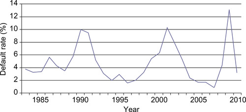 |
| Figure 12.2 Annual average corporate default rates for speculative grade firms, 1983–2010. Notes: The figure shows the annual default rates for firms rated speculative grade by Moody's. The data is from Moody's (2011). |
Figure 12.2 shows that the default rate is not constant over time—it is quite variable and seems highly persistent. The default rate alternates between periods of low default rates and periods with large spikes as happened for example during the recent financial crisis in 2007 to 2009.
The average corporate default rate for speculative grade (to be defined later) firms was 2.78% per year during the entire 1920–2010 period for which Moody's has data. For investment grade firms the average was just 0.15% per year.
Figure 12.3 shows the cumulative default rates over a 1- through 20-year horizon plotted for investment grade, speculative grade, and all firms.
 |
| Figure 12.3 Average cumulative global default rates. Notes: The figure shows the cumulative (over the horizon in years) average global default rates for investment grade, speculative grade, and all firms. The rates are calculated using data from 1920 to 2010. The data is from Moody's (2011). |
For example, the five-year cumulative default rate for all firms is 7.2%, which means historically there was a 7.2% probability of a firm defaulting during a five-year period. Over a 20-year horizon there is an 8.4% probability of an investment grade firm to default but a 41.4% probability of a speculative grade firm to default. The overall default rate is close to 18% for a 20-year horizon. The cumulative default rates are computed using data from 1920 through 2010.
These empirical default rates are not only of historical interest—they can also serve as useful estimates of the parameters in the credit portfolio risk models we study later.
3. Modeling Corporate Default
This section introduces the Merton model of corporate default, which provides important insights into the valuation of equity and debt when the probability of default is nontrivial. The model also helps us understand which factors affect the default probability.
Consider the situation where we are exposed to the risk that a particular firm defaults. This risk could arise from the fact that we own stock in the firm, or it could be that we have lent the firm cash, or it could be because the firm is a counterparty in a derivative transaction with us. We would like to use observed stock price on the firm to assess the probability of the firm defaulting.
Assume that the balance sheet of the company in question is of a particularly simple form. The firm is financed with debt and equity and all the debt expires at time t + T. The face value of the debt is D and it is fixed. The future asset value of the firm, At + T, is uncertain.
3.1. Equity Is a Call Option on the Assets of the Firm
At time t + T when the company's debt comes due the firm will continue to operate if  but the firm's debt holders will declare the firm bankrupt if
  and the firm will go into default. The stock holders of the firm are the residual claimants on the firm and to the stock holders the firm is therefore worth
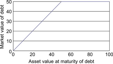
Figure 12.4 shows the value of firm equity Et + T as a function of the asset value At + T at maturity of the debt when the face value of debt D is $50.
 |
| Figure 12.4 |
The equity holder of a company can therefore be viewed as holding a call option on the asset value of the firm. It is important to note that in the case of stock options in Chapter 10 the stock price was the risky variable. In the present model of default, the asset value of the firm is the risky variable but the risky equity value can be derived as an option on the risky asset value.
The BSM formula in Chapter 10 can be used to value the equity in the firm in the Merton model. Assuming that asset volatility, σA, and the risk-free rate, rf, are constant, and assuming that the log asset value is normally distributed we get the current value of the equity to be
Recall from Chapter 10 and Chapter 11 that investors who are long options are long volatility. The Merton model therefore provides the additional insight that equity holders are long asset volatility. The option value is particularly large when the option is at-the-money; that is, when the asset value is close to the face value of debt. In this case if the manager holds equity he or she has an incentive to increase the asset value volatility (perhaps by taking on more risky projects) so as to increase the option value of equity. This action is not in the interest of the debt holders as we shall see now.
3.2. Corporate Debt Is a Put Option Sold
The simple accounting identity states that the asset value must equal the sum of debt and equity at any point in time and so we have
 |
| Figure 12.5 |
Comparing Figure 12.5 with the option payoffs in Chapter 10 we see that the debt holders look as if they have sold a put option although the out-of-the-money payoff has been lifted from 0 to $50 on the vertical axis corresponding to the face value of debt in this example.
Figure 12.5 suggests that we can rewrite the debt holder payoff as
Using the put option formula from Chapter 10 the value today of the corporate debt with face value D is

The debt holder is short a put option and so is short asset volatility. If the manager takes actions that increase the asset volatility of the firm, then the debt holders suffer because the put option becomes more valuable.
3.3. Implementing the Model
Recall from Chapter 10 that the stock return volatility needed to be estimated for the BSM model to be implemented. In order to implement the Merton model we need values for σA and At, which are not directly observable. In practice, if the stock of the firm is publicly traded then we do observe the number of shares outstanding and we also observe the stock price, and we therefore do observe Et,
Note that a crucially powerful feature of the Merton model is that we can use it to price corporate debt on firms even without observing the asset value as long as the stock price is available.
3.4. The Risk-Neutral Probability of Default
The risk-neutral probability of default in the Merton model corresponds in Chapter 10 to the probability that the put option is exercised. It is simply
It is important to note that this probability of default is constructed from the risk-neutral distribution (where assets grow at the risk-free rate rf) of asset values and so it may well be different from the actual (unobserved) physical probability. The physical default probability could be derived in the model but would require an estimate of the physical growth rate of firm assets.
Default risk is also sometimes measured in terms of distance to default, which is defined as
4. Portfolio Credit Risk
The Merton model gives powerful intuition about corporate default and debt pricing and it enables us to link the debt value to equity price and volatility, which in the case of public companies can be observed or estimated. While much can be learned from the Merton model, we have several motivations for going further.
• First, we are interested in studying the portfolio implications of credit risk. Default is a highly nonlinear event and furthermore default is correlated across firms and so credit risk is likely to impose limits on the benefits to diversification.
• Second, certain credit derivatives, such as collateralized debt obligations (CDOs), depend on the correlation of defaults that we therefore need to model.
• Third, for privately held companies we may not have the information necessary to implement the Merton model.
• Fourth, even if we have the information needed, for a portfolio of many loans, the implementation of Merton's model for each loan would be cumbersome.
In order to keep things relatively simple we will assume a single factor model similar to the market index model discussed in Chapter 7. For simplicity, we will also assume the normal distribution acknowledging that for risk management the use of the normal distribution is questionable at best.
We will assume a multivariate version of Merton's model in which the asset value of firm i is log normally distributed
We will assume further that the unconditional probability of default on any one loan is PD. This implies that the distance to default is now
We will assume that the horizon of interest, T, is one year so that T = 1 and T is therefore left out of the formulas in this section. For ease of notation we will also suppress the time subscripts, t, in the following.
4.1. Factor Structure
The relationship between asset values across firms will be crucial for measuring portfolio credit risk. Assume that the correlation between any firm i and any other firm j is ρ, which does not depend on i nor j. This equi-correlation assumption implies a factor structure on the n asset values. We have
Using the factor structure we can solve for  in terms of zi and F as
The probability of firm i defaulting conditional on the common factor F is therefore
4.2. The Portfolio Loss Rate Distribution
Define the gross loss (before recovery) when firm i defaults to be Li. Assuming that all loans are of equal size, relative loan size will not matter, and we can simply assume that
The credit portfolio loss rate is defined as the average of the individual losses via
The factor structure assumed earlier implies that conditional on F the Li variables are independent. This allows the distribution of the portfolio loss rate to be derived. It is only possible to derive the exact distribution when assuming that the number of firms, n, is infinite. The distribution is therefore only likely to be accurate in portfolios of many relatively small loans.
As the number of loans goes to infinity we can derive the limiting CDF of the loss rate L to be
The corresponding PDF of the portfolio loss rate is
Figure 12.6 shows the PDF of the loan loss rate when ρ = 0.10 and PD = 0.02.
 |
| Figure 12.6 |
Figure 12.6 clearly illustrates the nonnormality of the credit portfolio loss rate distribution. The loss distribution has large positive skewness that risk-averse investors will dislike. Recall from previous chapters that investors dislike negative skewness in the return distribution—equivalently they dislike positive skewness in the loss distribution.
The credit portfolio distribution in Figure 12.6 is not only important for credit risk measurement but it can also be used to value credit derivatives with multiple underlying assets such as collateralized debt obligations (CDOs), which were popular until the recent financial crisis.
4.3. Value-at-Risk on Portfolio Loss Rate
The VaR for the portfolio loss rate can be computed by inverting the CDF of the portfolio loss rate defined as FL (x) earlier. Because we are now modeling losses and not returns, we are looking for a loss VaR with probability (1 − p), which corresponds to a return VaR with probability p used in previous chapters.
We need to solve for  in
in
Figure 12.7 shows the  as a function of ρ for various values of PD. Recall from the definitions of Li and L that the loan loss rate can be at most 1 and so the VaR is restricted to be between 0 and 1 in this model.
 |
| Figure 12.7 |
Not surprisingly, Figure 12.7 shows that the VaR is higher when the default probability PD is higher. The effects of asset value correlation on VaR are more intriguing. Generally, an increasing correlation implies loss of diversification and so does an increasing VaR, but when PD is low (0.5%) and the correlation is high, then a further increase in correlation actually decreases the VaR slightly. The effect of correlation on the distribution is clearly nonlinear.
4.4. Granularity Adjustment
The model may appear to be restrictive because we have assumed that the n loans are of equal size. But it is possible to show that the limiting loss rate distribution is the same even when the loans are not of the same same size as long as the portfolio is not dominated by a few very large loans.
The limiting distribution, which assumes that n is infinite, can of course only be an approximation in any real-life applications where n is finite. It is possible to derive finite-sample refinements to the limiting distribution based on so-called granularity adjustments. Granularity adjustments for the VaR can be derived as well. For the particular model earlier, the granularity adjustment for the VaR is

The granularity adjusted VaR can now be computed as
Figure 12.8 shows the granularity adjustment GA (1 − p) corresponding to the VaRs in Figure 12.7.

It is clear from Figure 12.8 that the granularity adjustment is positive so that if we use the VaR that assumes infinitely many loans then we will tend to underestimate the true VaR. Figure 12.8 shows that the granularity adjustment is the largest when ρ is the smallest. The figure also shows that the adjustment is largest when the default probability, PD, is the largest.
5. Other Aspects of Credit Risk
5.1. Recovery Rates
In the case of default part of the face value is typically recovered by the creditors. When assessing credit risk it is therefore important to have an estimate of the expected recovery rate. Moody's defines recovery using the market prices of the debt 30 days after the date of default. The recovery rate is then computed as the ratio of the post-default market price to the face value of the debt.
Figure 12.9 shows the average (issuer-weighted) recovery rates for investment grade, speculative grade, and all defaults. The figure is constructed for senior-unsecured debt only. The two-year recovery rate for speculative grade firms is  . This number shows the average recovery rate on speculative grade issues that default at some time within a two-year period. The defaults used in Figure 12.9 are from the 1982 to 2010 period.

Figure 12.9 shows that the average recovery rate is around 40% for senior unsecured debt. Sometimes the loss given default (LGD) is reported instead of the recovery rate (RR). They are related via the simple identity LGD = 1 − RR.
If we are willing to assume a constant proportional default rate across loans then we can compute the credit portfolio $VaR taking into account recovery rates using
Figure 12.2 showed that the default rate varied strongly with time. This has not been built into our static factor model for portfolio credit risk but it could be by allowing for the factor F to change over time.
We may also wonder if the recovery rate over time is correlated with default rate. Figure 12.10 shows that it is negatively correlated in the data. The higher the default rate the lower the recovery rate.

Stochastic recovery and its correlation with default present additional sources of credit risk that have not been included in our simple model but that could be built in. In more complicated models, the VaR can be computed only via Monte Carlo simulation techniques such as those developed in Chapter 8.
5.2. Credit Quality Dynamics
The credit quality of a company typically declines well before any eventual default. It is important to capture this change in credit quality because the lower the quality the higher the chance of subsequent default.
One way to quantify the change in credit quality is by using the credit ratings provided by agencies such as Standard & Poor's and Moody's. The following list shows the ratings scale used by Moody's for long-term debt ordered from highest to lowest credit quality.
Investment Grades
• Aaa: Judged to be of the highest quality, with minimal credit risk.
• Aa: Judged to be of high quality and are subject to very low credit risk.
• A: Considered upper-medium grade and are subject to low credit risk.
• Baa: Subject to moderate credit risk. They are considered medium grade and as such may possess certain speculative characteristics.
Speculative Grades
• Ba: Judged to have speculative elements and are subject to substantial credit risk.
• B: Considered speculative and are subject to high credit risk.
• Caa: Judged to be of poor standing and are subject to very high credit risk.
• Ca: Highly speculative and are likely in, or very near, default, with some prospect of recovery of principal and interest.
• C: The lowest rated class of bonds and are typically in default, with little prospect for recovery of principal or interest.
Table 12.2 shows a matrix of one-year transition rates between Moody's ratings. The number in each cell corresponds to the probability that a company will transition from the row rating to the column rating in a year. For example, the probability of a Baa rated firm getting downgraded to Ba is 4.112%.
| Notes: The table shows Moody's credit rating transition rates estimated on annual data from 1970 through 2010. Each row represents last year's rating and each column represents this year's rating. Ca_C combines two rating categories. WR refers to withdrawn rating. Data is from Moody's (2011). | ||||||||||
| From/To | Aaa | Aa | A | Baa | Ba | B | Caa | Ca_C | WR | Default |
|---|---|---|---|---|---|---|---|---|---|---|
| Aaa | 87.395% | 8.626% | 0.602% | 0.010% | 0.027% | 0.002% | 0.002% | 0.000% | 3.336% | 0.000% |
| Aa | 0.971% | 85.616% | 7.966% | 0.359% | 0.045% | 0.018% | 0.008% | 0.001% | 4.996% | 0.020% |
| A | 0.062% | 2.689% | 86.763% | 5.271% | 0.488% | 0.109% | 0.032% | 0.004% | 4.528% | 0.054% |
| Baa | 0.043% | 0.184% | 4.525% | 84.517% | 4.112% | 0.775% | 0.173% | 0.019% | 5.475% | 0.176% |
| Ba | 0.008% | 0.056% | 0.370% | 5.644% | 75.759% | 7.239% | 0.533% | 0.080% | 9.208% | 1.104% |
| B | 0.010% | 0.034% | 0.126% | 0.338% | 4.762% | 73.524% | 5.767% | 0.665% | 10.544% | 4.230% |
| Caa | 0.000% | 0.021% | 0.021% | 0.142% | 0.463% | 8.263% | 60.088% | 4.104% | 12.176% | 14.721% |
| Ca_C | 0.000% | 0.000% | 0.000% | 0.000% | 0.324% | 2.374% | 8.880% | 36.270% | 16.701% | 35.451% |
The transition probabilities are estimated from the actual ratings changes during each year in the 1970–2010 period. The Ca_C category combines the companies rated Ca and C. The second-to-last column, which is labeled WR, denotes companies for which the rating was withdrawn. More interestingly, the right-most column shows the probability of a firm with a particular row rating defaulting within a year. Notice that the default rates are monotonically increasing as the credit ratings worsen. The probability of an Aaa rated firm defaulting is virtually zero whereas the probability of a Ca or C rated firm defaulting within a year is 35.451%.
Note also that for all the rating categories, the highest probability is to remain within the same category within the year. Ratings are thus persistent over time. The lowest rated firms have the least persistent rating. Many of them default or their ratings are withdrawn.
The rating transition matrices can be used in Monte Carlo simulations to generate a distribution of ratings outcomes for a credit risk portfolio. This can in turn be used along with ratings-based bond prices to compute the credit VaR of the portfolio. JP Morgan's CreditMetrics system for credit risk management is based on such an approach.
The credit risk portfolio model developed in Section 4 can also be extended to allow for debt value declines due to a deterioration of credit quality.
5.3. Credit Default Swaps
As discussed earlier, the price of corporate debt such as bonds is highly affected by the probability of default of the corporation issuing the debt. However, corporate bond prices are also affected by the prevailing risk-free interest rate as the Merton model showed us. Furthermore, in reality, corporate bonds are often relatively illiquid and so command a premium for illiquidity and illiquidity risk. Observed corporate bond prices therefore do not give a clean view of default risk. Fortunately, derivative contracts known as credit default swaps (CDS) that allow investors to trade default risk directly have appeared. CDS contracts give a pure market-based view of the default probability and its market price.
In a CDS contract the default protection buyer pays fixed quarterly cash payments (usually quoted in basis points per year) to the default protection seller. In return, in the event that the underlying corporation defaults, the protection seller will pay the protection buyer an amount equal to the par value of the underlying corporate bond minus the recovered value.
CDS contracts are typically quoted in spreads or premiums. A premium or spread of 200 basis points means that the protection buyer has to pay the protection seller 2% of the underlying face value of debt each year if a new CDS contract is entered into. Although the payments are made quarterly, the spreads are quoted in annual terms.
CDS contracts have become very popular because they allow the protection buyer to hedge default risk. They of course also allow investors to take speculative views on default risk as well as to arbitrage relative mispricings between corporate equity and bond prices.
Paralleling the developments in equity markets, CDS index contracts have developed as well. They allow investors to trade a basket of default risks using one liquid index contract rather than many illiquid firm-specific contracts.
Figure 12.11 shows the time series of CDS premia for two of the most prominent indices, namely the CDX NA (North American) and iTraxx EU (Europe). The CDX NA and iTraxx EU indexes each contain 125 underlying firms.
 |
| Figure 12.11 |
The data in Figure 12.11 are for five-year CDS contracts and the spreads are observed daily from March 20, 2007 through September 30, 2010. The financial crisis is painfully evident in Figure 12.11. Perhaps remarkably, unlike CDOs, trading in CDSs remained strong throughout the crisis and CDS contracts have become an important tool for managing credit risk exposures.
6. Summary
Credit risk is of fundamental interest to lenders but it is also of interest to investors who face counterparty default risk or investors who hold portfolios with corporate bonds or distressed equities.
This chapter has provided some important stylized facts on corporate default and recovery rates. We also developed a theoretical framework for understanding default based on Merton's seminal model. Merton's model studies one firm in isolation but it can be generalized to a portfolio of firms using Vasicek's factor model structure. The factor model can be used to compute VaR in credit portfolios. The chapter also briefly discussed credit default swaps, which are the financial instruments most closely linked with default risk.
Further Resources
This chapter has presented only some of the basic ideas and models in credit risk analysis. Hull (2008) discusses in detail credit risk management in banks. See Lando (2004) for a thorough treatment of credit risk models.
Merton (1974) developed the single-firm model in Section 3 and Vasicek (2002) developed the factor model in Section 4. The default and recovery data throughout the chapter is from Moody's, 2009 and Moody's, 2011.
Many researchers have developed extensions to the basic Merton model. Chapter 2 in Lando (2004) provides an excellent overview that includes Mason and Bhattacharya (1981) and Zhou (2001), who allow for jumps in the asset value. Hull et al. (2004) show that Merton's model can be extended so as to allow for the smirks in option-implied equity volatility that we saw in Chapter 10.
This chapter did not cover the so-called Z-scores from Altman (1968), who provides an important empirical approach to default prediction using financial ratios in a discriminant analysis.
The static and normal one-factor portfolio credit risk model in Section 4 can also be extended in several ways. Gagliardini and Gourieroux, 2011a and Gagliardini and Gourieroux, 2011b survey alternatives that include adding factors, allowing for nonnormality, and allowing for dynamic factors to capture default dynamics. The granularity adjustments have been studied in Gordy (2003), Gordy and Lutkebohmert (2007) and Gourieroux and Monfort (2010) and are based on the sensitivity analysis of VaR in Gourieroux et al. (2000).
Gordy (2003) studies credit risk models from a regulatory perspective. Basel Committee on Banking Supervision, 2001 and Basel Committee on Banking Supervision, 2003 contains the regulatory framework for ratings-based capital requirements.
Gordy (2000) provides a useful comparison of the two main credit portfolio risk models developed in industry, namely CreditRisk+ from Credit Suisse (1997) and CreditMetrics from JP Morgan (1997).
Jacobs and Li (2008) investigate corporate bond prices allowing for dynamic volatility of the form we studied in Chapter 4. The empirical relationship between asset correlation and default has been investigated by Lopez (2004). Karoui (2007) develops a model that allows for stochastic recovery rates. Christoffersen et al. (2009) study empirically the dynamic dependence of default.
References
Altman, E., Financial ratios: Discriminant analysis, and the prediction of corporate bankruptcy, J. Finance 23 (1968) 589–609.
Basel Committee on Banking Supervision, The New Basel Capital Accord, Consultative Document of the Bank for International Settlements, Part 2: Pillar 1, Available from:www.bis.org (2001).
Basel Committee on Banking Supervision, The New Basel Capital Accord, Consultative Document of the Bank for International Settlements, Part 3: The Second Pillar, Available from:www.bis.org (2003).
Christoffersen, P.; Ericsson, J.; Jacobs, K.; Jin, X., Exploring Dynamic Default Dependence, Available from: SSRN,http://ssrn.com/abstract=1400427 (2009).
Credit Suisse, CreditRisk+: A Credit Risk Management Framework, Credit Risk Financial Products, Available from:www.csfb.com (1997).
Gagliardini, P.; Gourieroux, C., Granularity Theory with Application to Finance and Insurance. (2011) University of Toronto; Manuscript.
Gagliardini, P.; Gourieroux, C., Granularity Adjustment for Risk Measures: Systematic vs. Unsystematic Risk. (2011) University of Toronto; Manuscript.
Gordy, M., A comparative anatomy of credit risk models, J. Bank. Finance 24 (2000) 119–149.
Gordy, M., A risk-factor model foundation for ratings-based bank capital rules, J. Financ. Intermed. 12 (2003) 199–232.
Gordy, M.; Lutkebohmert, E., Granularity Adjustment for Basel II (2007); Deutsche Bundesbank Discussion Paper.
Gourieroux, C.; Laurent, J.; Scaillet, O., Sensitivity analysis of values at risk, J. Empir. Finance 7 (2000) 225–245.
Gourieroux, C.; Monfort, A., Granularity in a qualitative factor model, J. Credit Risk 5 (Winter 2009/10) (2010) 29–65.
Hull, J., Risk Management and Financial Institutions. second ed (2008) Prentice Hall, Upper Saddle River, New Jersey.
Hull, J.; Nelken, I.; White, A., Merton's model, credit risk and volatility skews, J. Credit Risk 1 (2004) 1–27.
Jacobs, K.; Li, X., Modeling the dynamics of credit spreads with stochastic volatility, Manag. Sci. 54 (2008) 1176–1188.
Karoui, L., Modeling defaultable securities with recovery risk, Available from: SSRN,http://ssrn.com/abstract=896026 (2007).
Lando, D., Credit Risk Modeling. (2004) Princeton University Press, Princeton, New Jersey.
Lopez, J., The empirical relationship between average asset correlation, firm probability of default and asset size, J. Financ. Intermed. 13 (2004) 265–283.
Mason, S.; Bhattacharya, S., Risky debt, jump processes, and safety covenants, J. Financ. Econ. 9 (1981) 281–307.
Merton, R., On the pricing of corporate debt: The risk structure of interest rates, J. Finance 29 (1974) 449–470.
Moody's, Corporate Default and Recovery Rates, 1920–2008, Special Comment, Moody's. Available from:www.moodys.com (2009).
Moody's, Corporate Default and Recovery Rates, 1920–2010, Special Comment, Moody's. Available from:www.moodys.com (2011).
Morgan, J.P., CreditMetrics, Technical Document, Available from:http://www.msci.com/resources/technical_documentation/CMTD1.pdf (1997).
Vasicek, O., Loan portfolio value, Risk December (2002) 160–162.
Zhou, C., The term structure of credit spreads with jump risk, J. Bank. Finance 25 (11) (2001) 2015–2040.
1. Use the AR(1) model from Chapter 3 to model the default rate in Figure 12.2. What does the AR(1) model reveal regarding the persistence of the default rate? Can you fit the default rate closely? What is the fit (in terms of R2) of the AR(1) model?
2. Consider a company with assets worth $100 and a face value of debt of $80. The log return on government debt is 3%. If the company debt expires in two years and the asset volatility is 80% per year, then what is the current market value of equity and debt?
3. Assume that a company has 100,000 shares outstanding and that the stock is trading at $8 with a stock price volatility of 50% per year. The company has $500,000 in debt (face value) that matures in six months. The risk-free rate is 3%. Solve for the asset value and the asset volatility of the firm. What is the distance to default and the probability of default? What is the market value of the debt?
5. Replicate Figure 12.6. How does the loss rate distribution change when the correlation changes?
The answers to these exercises can be found in the Chapter12Results.xlsx file on the companion site.
For more information see the companion site at http://www.elsevierdirect.com/companions/9780123744487
..................Content has been hidden....................
You can't read the all page of ebook, please click here login for view all page.