
4. Volatility Modeling Using Daily Data
This chapter develops models for forecasting daily volatility when only daily return data are available. We first briefly describe the simplest variance models available including moving averages and the RiskMetrics variance model. We then introduce the GARCH variance model and compare it with the RiskMetrics model. We also suggest extensions to the basic GARCH model, which improve the model's ability to capture variance persistence and leverage effects. The GARCH model parameters must be estimated using the quasi-maximum likelihood method which is described in detail. Finally, we discuss tools for evaluating the performance of volatility forecasting models.
Keywords: Volatility, moving average, RiskMetrics, GARCH, leverage effect, quasi maximum likelihood
1. Chapter Overview
Part II of the book consists of three chapters. The ultimate goal of this and the following two chapters is to establish a framework for modeling the dynamic distribution of portfolio returns. The methods we develop in Part II can also be used to model each asset in the portfolio separately. In Part III of the book we will consider multivariate models that can link the univariate asset return models together. If the risk manager only cares about risk measurement at the portfolio level then the univariate models in Part II will suffice.
We will proceed with the univariate models in two steps. The first step is to establish a forecasting model for dynamic portfolio variance and to introduce methods for evaluating the performance of these forecasts. The second step is to consider ways to model nonnormal aspects of the portfolio return—that is, aspects that are not captured by the dynamic variance.
The second step, allowing for nonnormal distributions, is covered in Chapter 6. The first step, volatility modeling, is analyzed in this chapter and in Chapter 5. Chapter 5 relies on intraday data to develop daily volatility forecasts. The present chapter focuses on modeling daily volatility when only daily return data are available. We proceed as follows:
1. We briefly describe the simplest variance models available including moving averages and the so-called RiskMetrics variance model.
2. We introduce the GARCH variance model and compare it with the RiskMetrics model.
3. We estimate the GARCH parameters using the quasi-maximum likelihood method.
4. We suggest extensions to the basic model, which improve the model's ability to capture variance persistence and leverage effects. We also consider ways to expand the model, taking into account explanatory variables such as volume effects, day-of-week effects, and implied volatility from options.
5. We discuss various methods for evaluating the volatility forecasting models.
The overall objective of this chapter is to develop a general class of models that can be used by risk managers to forecast daily portfolio volatility using daily return data.
2. Simple Variance Forecasting
We begin by establishing some notation and by laying out the underlying assumptions for this chapter. In Chapter 1, we defined the daily asset log return, Rt + 1, using the daily closing price, St + 1, as
We will also apply the finding from Chapter 1 that at short horizons such as daily, we can safely assume that the mean value of Rt + 1 is zero since it is dominated by the standard deviation. Issues arising at longer horizons will be discussed in Chapter 8. Furthermore, we will assume that the innovation to asset return is normally distributed. We hasten to add that the normality assumption is not realistic, and it will be relaxed in Chapter 6. Normality is simply assumed for now, as it allows us to focus on modeling the conditional variance of the distribution.
Given the assumptions made, we can write the daily return as
Together these assumptions imply that once we have established a model of the time-varying variance,  we will know the entire distribution of the asset, and we can therefore easily calculate any desired risk measure. We are well aware from the stylized facts discussed in Chapter 1 that the assumption of conditional normality that is imposed here is not satisfied in actual data on speculative returns. However, as we will see later, for the purpose of variance modeling, we are allowed to assume normality even if it is strictly speaking not a correct assumption. This assumption conveniently allows us to postpone discussions of nonnormal distributions to a later chapter.
The focus of this chapter then is to establish a model for forecasting tomorrow's variance,  We know from Chapter 1 that variance, as measured by squared returns, exhibits strong autocorrelation, so that if the recent period was one of high variance, then tomorrow is likely to be a high-variance day as well. The easiest way to capture this phenomenon is by letting tomorrow's variance be the simple average of the most recent m observations, as in
Notice that this is a proper forecast in the sense that the forecast for tomorrow's variance is immediately available at the end of today when the daily return is realized. However, the fact that the model puts equal weights (equal to 1/m) on the past m observations yields unwarranted results. An extreme return (either positive or negative) today will bump up variance by 1/m times the return squared for exactly m periods after which variance immediately will drop back down. Figure 4.1 illustrates this point for m = 25 days. The autocorrelation plot of squared returns in Chapter 1 suggests that a more gradual decline is warranted in the effect of past returns on today's variance. Even if we are content with the box patterns, it is not at all clear how m should be chosen. This is unfortunate as the choice of m is crucial in deciding the patters of σt + 1: A high m will lead to an excessively smoothly evolving σt + 1, and a low m will lead to an excessively jagged pattern of σt + 1 over time.
 |
| Figure 4.1 |
JP Morgan's RiskMetrics system for market risk management considers the following model, where the weights on past squared returns decline exponentially as we move backward in time. The RiskMetrics variance model, or the exponential smoother as it is sometimes called, is written as
The RiskMetrics model has some clear advantages. First, it tracks variance changes in a way that is broadly consistent with observed returns. Recent returns matter more for tomorrow's variance than distant returns as λ is less than one and therefore the impact of the lagged squared return gets smaller when the lag, τ, gets bigger. Second, the model only contains one unknown parameter, namely, λ. When estimating λ on a large number of assets, RiskMetrics found that the estimates were quite similar across assets, and they therefore simply set λ = 0.94 for every asset for daily variance forecasting. In this case, no estimation is necessary, which is a huge advantage in large portfolios. Third, relatively little data need to be stored in order to calculate tomorrow's variance. The weight on today's squared returns is (1 − λ) = 0.06, and the weight is exponentially decaying to (1 − λ)λ99 = 0.000131 on the 100th lag of squared return. After including 100 lags of squared returns, the cumulated weight is  so that 99.8% of the weight has been included. Therefore it is only necessary to store about 100 daily lags of returns in order to calculate tomorrow's variance,
  .
.
Given all these advantages of the RiskMetrics model, why not simply end the discussion on variance forecasting here and move on to distribution modeling? Unfortunately, as we will see shortly, the RiskMetrics model does have certain shortcomings, which will motivate us to consider slightly more elaborate models. For example, it does not allow for a leverage effect, which we considered a stylized fact in Chapter 1 and it also provides counterfactual longer-horizon forecasts.
3. The GARCH Variance Model
We now introduce a set of models that capture important features of returns data and that are flexible enough to accommodate specific aspects of individual assets. The downside of these models is that they require nonlinear parameter estimation, which will be discussed subsequently.
The simplest generalized autoregressive conditional heteroskedasticity (GARCH) model of dynamic variance can be written as

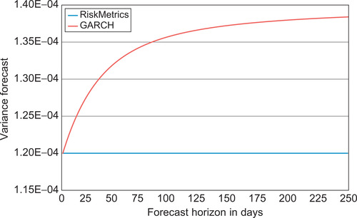
Our intuition might tell us that ignoring the long-run variance, as the RiskMetrics model does, is more important for longer-horizon forecasting than for forecasting simply one day ahead. This intuition is correct, as we will now see.
A key advantage of GARCH models for risk management is that the one-day forecast of variance,  is given directly by the model by
  . Consider now forecasting the variance of the daily return k days ahead, using only information available at the end of today. In GARCH, the expected value of future variance at horizon k is

We will refer to α + β as the persistence of the model. A high persistence—that is, an (α + β) close to 1—implies that shocks that push variance away from its long-run average will persist for a long time, but eventually the long-horizon forecast will be the long-run average variance, σ2. Similar calculations for the RiskMetrics model reveal that
So far we have considered forecasting the variance of daily returns k days ahead. Of more immediate interest is probably the forecast of variance of K-day cumulative returns,
The GARCH and RiskMetrics models share the inconvenience that the multiperiod distribution is unknown even if the one-day ahead distribution is assumed to be normal, as we do in this chapter. Thus, while it is easy to forecast longer-horizon variance in these models, it is not as easy to forecast the entire conditional distribution. We will return to this important issue in Chapter 8 since it is unfortunately often ignored in risk management.
4. Maximum Likelihood Estimation
In the previous section, we suggested a GARCH model that we argued should fit the data well, but it contains a number of unknown parameters that must be estimated. In doing so, we face the challenge that the conditional variance,  is an unobserved variable, which must itself be implicitly estimated along with the parameters of the model, for example, α, β, and ω.
4.1. Standard Maximum Likelihood Estimation
We will briefly discuss the method of maximum likelihood estimation, which can be used to find parameter values. Explicitly worked out examples are included in the answers to the empirical exercises contained on the web site.
A natural way to choose parameters to fit the data is then to maximize the joint likelihood of our observed sample. Recall that maximizing the logarithm of a function is equivalent to maximizing the function itself since the logarithm is a monotone, increasing function. Maximizing the logarithm is convenient because it replaces products with sums. Thus, we choose parameters (α, β, …), which solve
The MLE approach has the desirable property that as the sample size T goes to infinity the parameter estimates converge to their true values and the variance of these estimates are the smallest possible. In reality we of course do not have an infinite past of data available. Even if we have a long time series, say, of daily returns on the S&P 500 index available, it is not clear that we should use all that data when estimating the parameters. Sometimes obvious structural breaks such as a new exchange rate arrangement or new rules regulating trading in a particular market can guide in the choice of sample length. But often the dates of these structural breaks are not obvious and the risk manager is left with having to weigh the benefits of a longer sample, which implies more precise estimates (assuming there are no breaks), and a shorter sample, which reduces the risk of estimating across a structural break. When estimating GARCH models, a fairly good general rule of thumb is to use at least the past 1,000 daily observations and to update the estimate sample fairly frequently, say monthly.
4.2. Quasi-Maximum Likelihood Estimation
The skeptical reader will immediately protest that the MLEs rely on the conditional normal distribution assumption, which we argued in Chapter 1 is false. While this protest appears to be valid, a key result in econometrics says that even if the conditional distribution is not normal, MLE will yield estimates of the mean and variance parameters that converge to the true parameters, when the sample gets infinitely large as long as the mean and variance functions are properly specified. This convenient result establishes what is called quasi-maximum likelihood estimation (QMLE), referring to the use of normal MLE estimation even when the normal distribution assumption is false. Notice that QMLE buys us the freedom to worry about the conditional distribution later (in Chapter 6), but it does come at a price: The QMLE estimates will in general be less precise than those from MLE. Thus, we trade theoretical asymptotic parameter efficiency for practicality.
The operational aspects of parameter estimation will be discussed in the exercises following this chapter. Here we just point out one simple but useful trick, which is referred to as variance targeting. Recall that the simple GARCH model can be written as
4.3. An Example
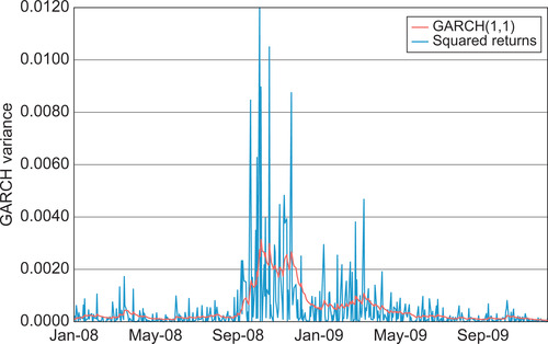
Figure 4.3 shows the S&P 500 squared returns from Figure 4.1, but now with an estimated GARCH variance superimposed. Using numerical optimization of the likelihood function (see the exercises at the end of the chapter), the optimal parameters imply the following variance dynamics:
 |
| Figure 4.3 |
The persistence of variance in this model is α + β = 0.999, which is only slightly lower than in RiskMetrics where it is 1. However, even if small, this difference will have consequences for the variance forecasts for horizons beyond one day. Furthermore, this very simple GARCH model may be misspecified driving the persistence close to one. We will consider more flexible models next.
5. Extensions to the GARCH Model
As we noted earlier, one of the distinct benefits of GARCH models is their flexibility. In this section, we explore this flexibility and present some of the models most useful for risk management.
5.1. The Leverage Effect
We argued in Chapter 1 that a negative return increases variance by more than a positive return of the same magnitude. This was referred to as the leverage effect, as a negative return on a stock implies a drop in the equity value, which implies that the company becomes more highly levered and thus more risky (assuming the level of debt stays constant). We can modify the GARCH models so that the weight given to the return depends on whether the return is positive or negative in the following simple manner:
Notice that it is strictly speaking a positive piece of news, zt > 0, rather than raw return Rt, which has less of an impact on variance than a negative piece of news, if θ > 0. The persistence of variance in this model is α(1 + θ2) + β, and the long-run variance is σ2 = ω/(1 − α(1 + θ2) − β).
Another way of capturing the leverage effect is to define an indicator variable, It, to take on the value 1 if day t's return is negative and zero otherwise.
A different model that also captures the leverage is the exponential GARCH model or EGARCH,
5.2. More General News Impact Functions
Allowing for a leverage effect is just one way to extend the basic GARCH model. Many extensions are motivated by generalizing the way in which today's shock to return, zt, impacts tomorrow's variance,  . This relationship is referred to as the variance news impact function, NIF. In general we can write
A very general news impact function can be defined by

5.3. More General Dynamics
The simple GARCH model discussed earlier is often referred to as the GARCH(1,1) model because it relies on only one lag of returns squared and one lag of variance itself. For short-term variance forecasting, this model is often found to be sufficient, but in general we can allow for higher order dynamics by considering the GARCH(p, q) model, which simply allows for longer lags as follows:
These higher-order GARCH models have the disadvantage that the parameters are not easily interpretable. The component GARCH structure offers a great improvement in this regard. Let us go back to the GARCH(1,1) model to motivate earlier we can use σ2 = ω/(1 − α − β) to rewrite the GARCH(1,1) model as
The component model can potentially capture autocorrelation patterns in variance, which die out slower than what is possible in the simple shorter-memory GARCH(1,1) model. Appendix A shows that the component model can be rewritten as a GARCH(2,2) model:
But the component GARCH structure has the advantage that it is easier to interpret its parameters and therefore also easier to come up with good starting values for the parameters than in the GARCH(2,2) model. In the component model ασ + βσ capture the persistence of the short-run variance component and αv + βv capture the persistence in the long-run variance component. The GARCH(2,2) dynamic parameters α1, α2, β1, β2 have no such straightforward interpretation.
The component model dynamics can be extended with a leverage or an even more general news impact function as discussed earlier in the case of GARCH(1,1).
The HYGARCH model is a different model, which explicitly allows for long-memory, or hyperbolic decay, rather than exponential decay in variance. When modeling daily data, long memory in variance might often be relevant and it may be helpful in forecasting at longer horizons, say beyond a week. Consult Appendix B at the end of the chapter for information on the HYGARCH model, which is somewhat more complicated to implement.
5.4. Explanatory Variables
Because we are considering dynamic models of daily variance, we have to be careful with days where no trading takes place. It is widely recognized that days that follow a weekend or a holiday have higher variance than average days. As weekends and holidays are perfectly predictable, it makes sense to include them in the variance model. Other predetermined variables could be yesterday's trading volume or prescheduled news announcement dates such as company earnings and FOMC meetings dates. As these future events are known in advance, we can model
We have not yet discussed option prices, but it is worth mentioning here that so-called implied volatilities from option prices often have quite high predictive value in forecasting next-day variance. Including the variance index (VIX) from the Chicago Board Options Exchange as an explanatory variable can improve the fit of a GARCH variance model of the underlying stock index significantly. Of course, not all underlying market variables have liquid options markets, so the implied volatility variable is not always available for variance forecasting. We will discuss the use of implied volatilities from options further in Chapter 10.
In general, we can write the GARCH variance forecasting model as follows:
5.5. Generalizing the Low Frequency Variance Dynamics
These discussions of long memory and of explanatory variables motivates us to consider another extension to the simple GARCH models referred to as Spline-GARCH models. The daily variances path captured by the simple GARCH models is clearly itself very volatile. Volatility often spikes up for a few days and then quickly reverts back down to normal levels. Such quickly reverting spikes make volatility appear noisy and thus difficult to capture by explanatory variables. Explanatory variables may nevertheless be important for capturing longer-term trends in variance, which may thus need to be modeled separately so as to not be contaminated by the daily spikes.
In addition, some speculative prices may exhibit structural breaks in the level of volatility. A country may alter its foreign exchange regime, and a company may take over another company, for example, which could easily change its volatility structure.
In order to capture low-frequency changes in volatility we generalize the simple GARCH(1,1) model to the following multiplicative structure:

The Spline-GARCH model captures low frequency dynamics in variance via the τt + 1 process, and higher-frequency dynamics in variance via the gt + 1 process. Notice that the low-frequency variance is kept positive via the exponential function. The low-frequency variance has a log linear time-trend captured by ω1 and a quadratic time-trend starting at time t0 and captured by ω2. The low-frequency variance is also driven by the explanatory variables in the vector Xt.
Notice that the long-run variance in the Spline-GARCH model is captured by the low-frequency process
We can generalize the quadratic trend by allowing for many, say l, quadratic pieces, each starting at different time points and each with different slope parameters:
5.6. Estimation of Extended Models
A particularly powerful feature of the GARCH family of models is that they can all be estimated using the same quasi MLE technique used for the simple GARCH(1,1) model. Regardless of the news impact functions, the dynamic structure, and the choice of explanatory variables, the model parameters can be estimated by maximizing the nontrivial part of the log likelihood
6. Variance Model Evaluation
Before we start using the variance model for risk management purposes, it is appropriate to run the estimated model through some diagnostic checks.
6.1. Model Comparisons Using LR Tests
We have seen that the basic GARCH model can be extended by adding parameters and explanatory variables. The likelihood ratio test provides a simple way to judge if the added parameter(s) are significant in the statistical sense. Consider two different models with likelihood values L0 and L1, respectively. Assume that model 0 is a special case of model 1. In this case we can compare the two models via the likelihood ratio statistic
The LR statistic will always be a positive number because model 1 contains model 0 as a special case and so model 1 will always fit the data better, even if only slightly so. The LR statistic will tell us if the improvement offered by model 1 over model 0 is statistically significant. It can be shown that the LR statistic will have a chi-squared distribution under the null hypothesis that the added parameters in model 1 are insignificant. If only one parameter is added then the degree of freedom in the chi-squared distribution will be 1. In this case the 1% critical value is approximately 6.63. A good rule of thumb is therefore that if the log-likelihood of model 1 is 3 to 4 points higher than that of model 0 then the added parameter in model 1 is significant. The degrees of freedom in the chi-squared test is equal to the number of parameters added in model 1.
6.2. Diagnostic Check on the Autocorrelations
In Chapter 1, we studied the behavior of the autocorrelation of returns and squared returns. We found that the raw return autocorrelations did not display any systematic patterns, whereas the squared return autocorrelations were positive for short lags and decreased as the lag order increased.
The objective of variance modeling is essentially to construct a variance measure,  , which has the property that the standardized squared returns,
  , have no systematic autocorrelation patterns. Whether this has been achieved can be assessed via the red line in Figure 4.5, where we show the autocorrelation of
  from the GARCH model with leverage for the S&P 500 returns along with their standard error bands. The standard errors are calculated simply as
  , where T is the number of observations in the sample. Usually the autocorrelation is shown along with plus/minus two standard error bands around zero, which simply mean horizontal lines at
  and
and  These so-called Bartlett standard error bands give the range in which the autocorrelations would fall roughly 95% of the time if the true but unknown autocorrelations of
  were all zero.

The blue line in Figure 4.5 redraws the autocorrelation of the squared returns from Chapter 1, now with the standard error bands superimposed. Comparing the two panels in Figure 4.5, we see that the GARCH model has been quite effective at removing the systematic patterns in the autocorrelation of the squared returns.
6.3. Volatility Forecast Evaluation Using Regression
Another traditional method of evaluating a variance model is based on simple regressions where squared returns in the forecast period, t + 1, are regressed on the forecast from the variance model, as in
First of all, notice that it is true that  so that the squared return is an unbiased proxy for true variance. But the variance of the proxy is
Due to the high degree of noise in the squared returns, the fit of the preceding regression as measured by the regression R2 will be very low, typically around 5% to 10%, even if the variance model used to forecast is indeed the correct one. Thus, obtaining a low R2 in such regressions should not lead us to reject the variance model. The conclusion is just as likely to be that the proxy for true but unobserved variance is simply very inaccurate.
In the next chapter we will look at ways to develop more accurate (realized volatility) proxies for daily variance using intraday return data.
6.4. The Volatility Forecast Loss Function
The ordinary least squares (OLS) estimation of a linear regression chooses the parameter values that minimize the mean squared error (MSE) in the regression. The regression-based approach to volatility forecast evaluation therefore implies a quadratic volatility forecast loss function. A correct volatility forecasting model should have b0 = 0 and b1 = 1 as discussed earlier. A sensible loss function for comparing volatility models is therefore
Risk managers may however care differently about a negative versus a positive volatility forecast error of the same magnitude: Underestimating volatility may well be more costly for a conservative risk manager than overestimating volatility by the same amount.
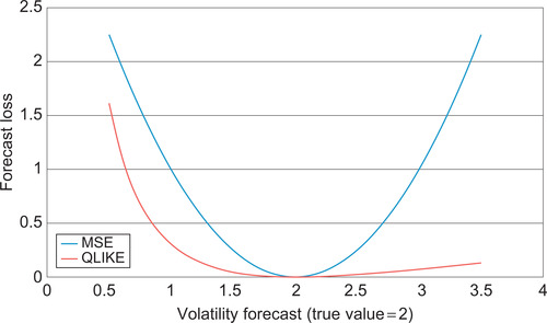
In order to evaluate volatility forecasts allowing for asymmetric loss, the following function can be used instead of MSE:
Notice that the QLIKE loss function depends on the relative volatility forecast error,  , rather than on the absolute error,
  ; which is the key ingredient in MSE. The QLIKE loss function will always penalize more heavily volatility forecasts that underestimate volatility.
In Figure 4.6 we plot the MSE and QLIKE loss functions when the true volatility is 2 and the volatility forecast ranges from 0 to 4. Note the strong asymmetry of QLIKE for negative versus positive volatility forecast errors.
 |
| Figure 4.6 |
It can be shown that the MSE and the QLIKE loss functions are both robust with respect to the choice of volatility proxy. A volatility forecast loss function is said to be robust if the ranking of any two volatility forecasts is the same when using an observed volatility proxy as when (hypothetically) using the unobserved true volatility. Robustness is clearly a desirable quality for a volatility forecast loss function. Essentially only the MSE and QLIKE functions possess this quality.
Note again that we have only considered the noisy squared return,  , as a volatility proxy. In the next chapter we will consider more precise proxies using intraday information.
7. Summary
This chapter presented a range of variance models that are useful for risk management. Simple equally weighted and exponentially weighted models that require minimal effort in estimation were first introduced. Their shortcomings led us to consider more sophisticated but still simple models from the GARCH family. We highlighted the flexibility of GARCH as a virtue and considered various extensions to account for leverage effects, day-of-week effects, announcement effects, and so on. The powerful and flexible quasi-maximum likelihood estimation technique was presented and will be used again in coming chapters. Various model validation techniques were introduced subsequently. Most of the techniques suggested in this chapter are put to use in the empirical exercises that follow.
This chapter focused on models where daily returns are used to forecast daily volatility. In some situations the risk manager may have intraday returns available when forecasting daily volatility. In this case more accurate models are available. These models will be analyzed in the next chapter.
Appendix A. Component GARCH and GARCH(2,2)
This appendix shows that the component GARCH model can be viewed as a GARCH(2,2) model. First define the lag operator, L, to be a function that transforms the current value of a time series to the lagged value, that is,


Appendix B. The HYGARCH Long-Memory Model
This appendix introduces the long-memory GARCH model of Davidson (2004), which he refers to as HYGARCH (where HY denotes hyperbolic). Consider first the standard GARCH(1,1) model where
We can show that when  ,
,  ,
,  , and
, and  we get the regular GARCH(1,1) model as a special case of the HYGARCH. When
  ,
, 
 , and
, and  we get the RiskMetrics model as a special case of HYGARCH.
The HYGARCH model can be estimated using MLE as well. Please refer to Davidson (2004) for more details on this model.
Further Resources
The literature on variance modeling has exploded during the past 30 years, and we only present a few examples of papers here. Andersen et al. (2007) contains a discussion of the use of volatility models in risk management. Evidence on the performance of GARCH models through the 2008–2009 financial crisis can be found in Brownlees et al. (2009).
Andersen et al. (2006) and Poon and Granger (2005) provide overviews of the various classes of volatility models. The exponential smoother variance model is studied in JP Morgan (1996). The exponential smoother has been used to forecast a wide range of variables and further discussion of it can be found in Granger and Newbold (1986). The basic GARCH model is introduced in Engle (1982) and Bollerslev (1986) and it is discussed further in Bollerslev et al. (1992) and Engle and Patton (2001). Engle (2002) introduces the GARCH model with exogenous variable. Bollerslev (2008) summarizes the many variations on the basic GARCH model.
Long memory including fractional integrated generalized autoregressive conditional heteroskedasticity (FIGARCH) models were introduced in Baillie et al. (1996) and Bollerslev and Mikkelsen (1999). The hyperbolic HYGARCH model in Appendix B is developed in Davidson (2004).
Component volatility models were introduced in Engle and Lee (1999). They have been applied to option valuation in Christoffersen et al., 2010 and Christoffersen et al., 2008. The Spline-GARCH model with a deterministic volatility component was introduced in Engle and Rangel (2008).
The leverage effect and other GARCH extensions are described in Ding et al. (1993), Glosten et al. (1993), Hentschel (1995) and Nelson (1990). Most GARCH models use squared return as the innovation to volatility. Forsberg and Ghysels (2007) analyze the benefits of using absolute returns instead.
Quasi maximum likelihood estimation of GARCH models is developed in Bollerslev and Wooldridge (1992). Francq and Zakoian (2009) survey more recent results. For practical issues involved in GARCH estimation see Zivot (2009). Hansen and Lunde (2005), Patton and Sheppard (2009) and Patton (2011) develop tools for volatility forecast evaluation and volatility forecast comparisons.
Taylor (1994) contains a very nice overview of a different class of variance models known as stochastic volatility models. This class of models was not included in this book due to the relative difficulty of estimating them.
Andersen, T.; Christoffersen, P.; Diebold, F., Volatility and correlation forecasting, In: (Editors: Elliott, G.; Granger, C.; Timmermann, A.) The Handbook of Economic Forecasting (2006) Elsevier, Amsterdam, The Netherlands, pp. 777–878.
Andersen, T.; Bollerslev, T.; Christoffersen, P.; Diebold, F., Practical volatility and correlation modeling for financial market risk management, In: (Editors: Carey, M.; Stulz, R.) The NBER Volume on Risks of Financial Institutions (2007) University of Chicago Press, Chicago, IL, pp. 513–548.
Baillie, R.; Bollerslev, T.; Mikkelsen, H., Fractionally integrated generalized autoregressive conditional heteroskedasticity, J. Econom. 74 (1996) 3–30.
Bollerslev, T., Generalized autoregressive conditional heteroskedasticity, J. Econom. 31 (1986) 307–327.
Bollerslev, T., Glossary to ARCH (GARCH), Available from: SSRNhttp://ssrn.com/abstract=1263250 (2008).
Bollerslev, T.; Chou, R.; Kroner, K., ARCH modeling in finance: A review of the theory and empirical evidence, J. Econom. 52 (1992) 5–59.
Bollerslev, T.; Mikkelsen, H., Long-term equity anticipation securities and stock market volatility dynamics, J. Econom. 92 (1999) 75–99.
Bollerslev, T.; Wooldridge, J., Quasi-maximum likelihood estimation and inference in dynamic models with time varying covariances, Econom. Rev. 11 (1992) 143–172.
Brownlees, C.; Engle, R.; Kelly, B., A Practical Guide to Volatility Forecasting through Calm and Storm, Available from: SSRNhttp://ssrn.com/abstract=1502915 (2009).
Christoffersen, P.; Dorion, C.; Jacobs, K.; Wang, Y., Volatility components: Affine restrictions and non-normal innovations, J. Bus. Econ. Stat. 28 (2010) 483–502.
Christoffersen, P.; Jacobs, K.; Ornthanalai, C.; Wang, Y., Option valuation with long-run and short-run volatility components, J. Financial Econ. 90 (2008) 272–297.
Davidson, J., Moment and memory properties of linear conditional heteroskedasticity models, and a new model, J. Bus. Econ. Stat. 22 (2004) 16–29.
Ding, Z.; Granger, C.W.J.; Engle, R.F., A long memory property of stock market returns and a new model, J. Empir. Finance 1 (1) (1993) 83–106.
Engle, R., Autoregressive conditional heteroskedasticity with estimates of the variance of U.K. inflation, Econometrica 50 (1982) 987–1008.
Engle, R., New frontiers in ARCH models, J. Appl. Econom. 17 (2002) 425–446.
Engle, R.; Lee, G., A permanent and transitory component model of stock return volatility, In: (Editors: Engle, R.; White, H.) Cointegration, Causality, and Forecasting: A Festschrift in Honor of Clive W.J. Granger (1999) Oxford University Press, New York, NY, pp. 475–497.
Engle, R.; Patton, A., What good is a volatility model?Quant. Finance 1 (2001) 237–245.
Engle, R.; Rangel, J., The spline-GARCH model for low-frequency volatility and its global macroeconomic causes, Rev. Financ. Stud. 21 (2008) 1187–1222.
Francq, C.; Zakoian, J.-M., A tour in the asymptotic theory of GARCH estimation, In: (Editors: Andersen, T.G.; Davis, R.A.; Kreib, J.-P.; Mikosch, Th.) Handbook of Financial Time Series (2009) Heidelberg, Germany, pp. 85–112.
Forsberg, L.; Ghysels, E., Why do absolute returns predict volatility so well?J. Financ. Econom. 5 (2007) 31–67.
Glosten, L.; Jagannathan, R.; Runkle, D., On the relation between the expected value and the volatility of the nominal excess return on stocks, J. Finance 48 (1993) 1779–1801.
Granger, C.W.J.; Newbold, P., Forecasting Economic Time Series. second ed (1986) Academic Press, New York.
Hansen, P.; Lunde, A., A forecast comparison of volatility models: Does anything beat a GARCH(1,1)?J. Appl. Econom. 20 (2005) 873–889.
Hentschel, L., All in the family: Nesting symmetric and asymmetric GARCH models, J. Financ. Econ. 39 (1995) 71–104.
Morgan, J.P., RiskMetrics-Technical Document. fourth ed (1996) J.P. Morgan/Reuters, New York, NY.
Nelson, D., Conditional heteroskedasticity in asset pricing: A new approach, Econometrica 59 (1990) 347–370.
Patton, A., Volatility forecast comparison using imperfect volatility proxies, J. Econom. 160 (2011) 246–256.
Patton, A.; Sheppard, K., Evaluating volatility and correlation forecasts, In: (Editors: Andersen, T.G.; Davis, R.A.; Kreiss, J.-P.; Mikosch, T.) Handbook of Financial Time Series (2009) Springer Verlag, Berlin.
Poon, S.; Granger, C., Practical issues in forecasting volatility, Financ. Analyst. J. 61 (2005) 45–56.
Taylor, S., Modelling stochastic volatility: A review and comparative study, Math. Finance 4 (1994) 183–204.
Zivot, E., Practical issues in the analysis of univariate GARCH models, In: (Editors: Andersen, T.G.; Davis, R.A.; Kreib, J.-P.; Mikosch, Th.) Handbook of Financial Time Series (2009) Springer Verlag, Berlin, pp. 113–156.
Open the Chapter4Data.xlsx file from the companion site.
A number of the exercises in this and the coming chapters rely on the maximum likelihood estimation (MLE) technique. The general approach to answering these questions is to use the parameter starting values to calculate the log likelihood value of each observation and then compute the sum of these individual log likelihoods. When using Excel, the Solver tool is then activated to maximize the sum of the log likelihoods by changing the cells corresponding to the parameter values. Solver is enabled through the Windows Office menu by selecting Excel Options and Add-Ins. When using Solver, choose the options Use Automatic Scaling and Assume Non-Negative. Set Precision, Tolerance, and Convergence to 0.0000001.
1. Estimate the simple GARCH(1,1) model on the S&P 500 daily log returns using the maximum likelihood estimation (MLE) technique. First estimate
2. Include a leverage effect in the variance equation. Estimate
3. Include the option implied volatility VIX series from the Chicago Board Options Exchange (CBOE) as an explanatory variable in the GARCH equation. Use MLE to estimate
4. Estimate the component GARCH model defined by
The answers to these exercises can be found in the Chapter4Results.xlsx file on the companion site.
For more information see the companion site at http://www.elsevierdirect.com/companions/9780123744487
..................Content has been hidden....................
You can't read the all page of ebook, please click here login for view all page.