Appendix B

SQL Extensions for Data Analysis

Unlike SQL:92 which provides limited aggregation functionality, SQL:1999 standard defines a rich set of aggregate functions. Most of these functions are supported by Oracle and IBM DB2, and other databases will support these functions in the near future. SQL:1999 provides some extensions to basic GROUP BY clause using ROLLUP and CUBE clauses. It also provides a set of new analytic functions that provide a means by which pivot reports and OLAP queries can be computed easily in nonprocedural SQL.

Prior to the introduction of analytic functions, complex reports could be produced in SQL by complex self-joins and nested queries, which were difficult to write and inefficient to execute. SQL analytic functions and extensions not only make queries easier to code but also make them faster than could be achieved with pure SQL or PL/SQL. This appendix discusses each of them in detail. It also introduces the concept of windowing in SQL:1999.

B.1 EXTENSIONS TO GROUP BY CLAUSE

SQL:1999 extends the GROUP BY clause to provide better support for rollup and cross-tab queries. SQL:1999 supports ROLLUP and CUBE constructs that are the generalizations of the GROUP BY clause. Both constructs are similar in functionality in a way that both of them return additional data in the result of the query when added to the GROUP BY clause. The only difference between the two clauses is that CUBE returns even more information than ROLLUP. To understand the ROLLUP and CUBE constructs, consider the following SQL query.

  SELECT bid, tid, SUM(Number) AS Total
  FROM SALES
  GROUP BY ROLLUP (bid, tid);

The SALES relation used in this query is shown in Figure 14.2. The result of this query is shown in Figure B.1. The three additional rows with null value in the tid column provide the total for each value (B1, B2, and B3) in the bid column. For example, additional row for B1 indicates the total books with bid B1 sold in all time periods. Note that the tid column includes a null value for these particular rows. Its value cannot be calculated as all three subgroups (from the tid column) are already represented. The last row shows that the bookshop has sold 413 books in total.

 

bid	tid	Total
B1	1	59
B1	2	47
B1	3	32
B1	NULL	138
B2	1	46
B2	2	38
B2	3	41
B2	NULL	125
B3	1	45
B3	2	43
B3	3	62
B3	NULL	150
NULL	NULL	413

Fig. B.1 Result of GROUP BY ROLLUP on SALES

In addition to attributes from the fact table (such as bid, tid, and lid), attributes from the dimension tables can be also specified in the rollup and cross-tab queries. For example, if the user wants to see the cross-tab on the category of the books and year instead of bid and tid, following SQL command can be given.

  SELECT Category, Year, SUM(Number) AS Total
  FROM BOOK B, SALES S, TIME T
  WHERE B.bid=S.bid AND T.tid=S.tid
  GROUP BY ROLLUP (Category, Year);

The result of the SQL query is given in Figure B.2. The result of this query provides the information that the bookshop has sold 138 textbooks, 125 language books, and 150 novels. The last row shows that bookshop has sold a total of 413 books.

If we replace the ROLLUP clause with the CUBE clause in our example SQL query, some more information is provided. For example, consider the following SQL query.

SELECT Category, Year, SUM(Number) AS Total

FROM BOOK B, SALES S, TIME T

WHERE B.bid = S.bid AND T.tid=S.tid

GROUP BY CUBE (Category, Year);

Category	Year	Total
Textbook	2006	59
Textbook	2007	79
Textbook	NULL	138
Language Book	2006	46
Language Book	2007	79
Language Book	NULL	125
Novel	2006	45
Novel	2007	105
Novel	NULL	150
NULL	NULL	413

Fig. B.2 Result of GROUP BY ROLLUP on SALES by Category and Year

The result of this query is shown in Figure B.3. Note that two more rows have been added to the query result—one for each different value in the Year Column. Unlike the ROLLUP clause, the CUBE clause gives the summarized information for each subgroup. A null value in the Category column indicates that all the three categories (Textbook, Language Book, and Novel) are included in each subgroup summary. The CUBE clause provides extra information that the bookshop has more sales in the year 2007 than in 2006. This information is not provided by the ROLLUP clause.

Grouping Function

As discussed earlier, SQL:1999 uses null to indicate both the unknown value as well as all. However, null values returned by the ROLLUP and CUBE are not always the stored null—instead, a null may indicate that the row contains a subtotal. Thus, a problem arises if the query results contain both the stored null and null created by a ROLLUP or CUBE. GROUPING function is used to distinguish the two null values. The function GROUPING is an aggregate function that returns 1 when it encounters a null value created by a CUBE or ROLLUP operation. Any other type of value, including a stored null, returns 0.

 

Category	Year	Total
Textbook	2006	59
Textbook	2007	79
Textbook	NULL	138
Language Book	2006	46
Language Book	2007	79
Language Book	NULL	125
Novel	2006	45
Novel	2007	105
Novel	NULL	150
NULL	2006	150
NULL	2007	263
NULL	NULL	413

Fig. B.3 Result of GROUP BY CUBE on SALES

For example, consider the following SQL query.

  SELECT Category, Year, SUM(Number) AS Total
  GROUPING(Category) AS c_flag,
  GROUPING(Year) AS y_flag
  FROM BOOK B, SALES S, TIME T
  WHERE B.bid=S.bid AND T.tid=S.tid
  GROUP BY ROllUP (Category, Year);

The result of this query is given in Figure B.4. The result contains two extra columns called c_flag and y_flag. In each tuple, these columns will contain 1 if the corresponding null value is generated by ROLLUP or CUBE, otherwise 0 in all other cases. A row with flag values ‘0 0’ indicates that it is a detailed row (row without the summary values). A row with flag values ‘0 1’ indicates that it is a first level subtotal row. The row with flag values ‘1 1’ indicates that it is a grand total row.

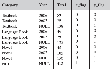
Fig. B.4 Result of GROUPING function

DECODE Function

The readability of the query result can be further improved by replacing the null value by a value of our choice. This can be done by using the GROUPING function with the DECODE function. For example, consider this SQL query.

  SELECT Category, Country,
  SUM(Number) AS Total
  DECODE (GROUPING(Category), 1, ‘All
  Categories’, Category),
  DECODE (GROUPING(Country), 1, ‘All
  Countries’, Country),
  FROM BOOK B, SALES S, LOCATION L
  WHERE B.bid=S.bid AND L.lid=S.lid
  GROUP BY CUBE (Category, Country);

In this query, the DECODE function returns the value ‘All Categories’ if the value of Category is a null generated by CUBE operator and returns the actual values otherwise. Similarly, it returns the value ‘All Countries’ if the value of Country is a null generated by CUBE operator and returns the actual values otherwise. The result is shown in Figure B.5.

 

Category	Country	Total
Textbook	India	85
Textbook	USA	53
Textbook	All Countries	138
Language Book	India	84
Language Book	USA	41
Language Book	All Countries	125
Novel	India	116
Novel	USA	34
Novel	All Countries	150
All Countries	India	285
All Countries	USA	128
All Countries	All Countries	413

Fig. B.5 Result of DECODE function

B.2 NEW ANALYTIC FUNCTIONS

SQL:1999 provides 33 new analytic functions. It supports standard deviation and variance functions (STDDEV and VARIANCE) which are applied on single attribute. Some of the database systems also support other aggregate functions such as median and mode. SQL:1999 also supports binary aggregate functions which can be applied on the pairs of attributes. These functions include correlations and covariance and regression curves (CORR, COVAR_POP, REGR_COUNT, etc.). Definitions of these functions may be found in any standard textbook on statistics. Thus, we will not discuss these functions in detail.

Analytic functions enable you to compute aggregate values for a specific group of rows. They differ from aggregate functions in a way that they return multiple rows for each group. Analytic functions are invoked using the OVER() clause which has three components.

• PARTITION BY clause, which divides the query result set into groups. If PARTITION BY clause is missing, the entire result set is treated as a single partition.
• ORDER BY clause, which sorts the query result set or the partition in ascending or descending order as specified.
• RANGE or ROWS clause, by which the function can be made to include values or rows around the current row in its calculations. These clauses are used in window queries.

This section discusses only the ranking and window aggregate functions provided by SQL:1999.

Ranking Functions

A ranking function computes the rank of a row compared to other rows in the result set. SQL:1999 provides four types of ranking functions.

• RANK and DENSE_RANK
• CUME_DIST and PERCENT_RANK
• ROW_NUMBER
• NTILE

The BOOK table shown in Figure B.6 is taken for illustration of these functions.

 

Book_title	Category	Price
C++	Textbook	40
Ransack	Novel	22
Learning French Language	Language Book	32
Differential Calculus	Textbook	32
Call Away	Novel	22
DBMS	Textbook	40
Introduction to German Language	Language Book	22
Coordinate Geometry	Textbook	35
UNIX	Textbook	26

Fig. B.6 BOOK table

RANK and DENSE_RANK Functions The RANK function returns a ranking value for each row in the query result set. Ranking is done in conjunction with an ORDER BY clause. For example, to find the rank of each book in the order of their price (the book with the highest price will get rank 1), following SQL query can be used.

SELECT Book_title, Price, RANK() OVER(ORDER BY Price DESC) AS b_rank FROM BOOK;

This query displays the book title, price, and rank assigned to each book according to its price. The output of this query is shown in Figure B.7(a). If there are multiple rows for a given value of the ordering attribute, the RANK function assigns the same rank to all the rows that have the same value of the ordering attribute. For example, if there are two books with the highest price, then both of them will get rank 1. The next row in the sequence will get rank 3 and not 2. Thus, RANK function leaves gaps in the ranking sequence in case of ties as shown in the output.

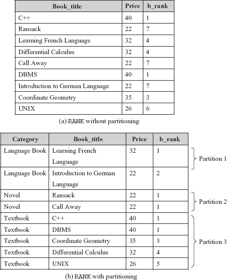
Fig. B.7 Output of query containing RANK function

Note that the rows in the output may not be sorted by rank, thus, an extra ORDER BY clause is required to get them sorted in the order of b_rank as shown in this SQL query.

SELECT Book_title, Price, RANK() OVER(ORDER BY Price DESC) AS b_rank FROM BOOK ORDER BY b_rank;

The DENSE_RANK function works similarly as RANK function, but it does not leave gaps in the ranking sequence. Thus, two books with highest price will get rank 1 and the next row will get rank 2 instead of 3. To understand the DENSE_RANK function, consider the following SQL query.

SELECT Book_title, Price, DENSE_RANK() OVER(ORDER BY Price DESC) AS b_rank FROM BOOK ORDER BY b_rank;

Ranking can also be done within the partitions of the result set. The partitions of the query result set can be created using the PARTITION BY clause. The PARTITION BY clause divides the query result set into partitions within which the RANK function is applied. The analytic functions such as RANK, DENSE_RANK, NTILE, ROW_NUMBER, etc., are applied to each partition independently. Thus, they are reset for each partition. For example, consider this SQL query.

SELECT Category, Book_title, Price, DENSE_RANK() OVER (PARTITION BY Category ORDER BY Price DESC) AS b_rank FROM BOOK ORDER BY Category, b_rank;

This SQL query first partitions the tuples on the basis of the attribute Category. It then assigns a rank to each book within the partition according to its price. The book with the highest price within the partition will get a rank 1. The outer ORDER BY clause orders the result tuples first by Category and within each category by b_rank. The output of this query is shown in Figure B.7(b). Note that within each partition, the rank starts with 1.

 

If null values are present in the table, one null value is assumed to be equal to another null value while calculating the rank. SQL:1999 allows the user to specify where to put null values in the query result set by using the NULLS FIRST or NULLS LAST clause. For example, consider this SQL query.

SELECT Book_title, Price, RANK() OVER(ORDER BY(Price) DESC NULLS LAST) AS ranking FROM BOOK;

PERCENT_RANK and CUME_DIST Functions The PERCENT_RANK function computes the rank of a row within each partition as a fraction. The PERCENT_RANK of a row can be calculated as

(rank of a row in its partition-1)/(number of rows being evaluated-1)

The number of rows being evaluated can be an entire query result set or a partition. This function will return null if there is only one tuple in the partition. For example, consider this SQL query.

SELECT Category, Book_title, Price, PERCENT_RANK() OVER (PARTITION BY Category ORDER BY Price DESC) AS p_rank FROM BOOK ORDER BY Category, p_rank;

It calculates the percent rank of the book’s price for each book within the category. The output of this query is given in Figure B.8(a).

Fig. B.8 Output of query containing PERCENT_RANK and CUME_DIST function

The CUME_DIST (cumulative distribution) uses the row count (number of rows in the partition with ordering values less than or equal to the ordering value of the tuple) instead of its rank value. The CUME_DIST can be calculated as

  (Row count)/(number of rows being evaluated)

For example, consider this SQL query.

SELECT Book_title, Price, CUME_DIST() OVER (PARTITION BY Category ORDER BY Price) AS c_rank FROM BOOK WHERE Category=‘Textbook’ ORDER BY Price;

This query calculates the price percentile of each book in the textbook category. The output of this query is given in Figure B.8(b).

ROW_NUMBER Function The ROW_NUMBER function sorts the tuples and assigns a unique number to each tuple (sequentially, starting with 1) according to its position in the sort order within the partition or in the entire query result set. For example, consider this SQL query.

SELECT Category, Book_title, Price, ROW_NUMBER() OVER (PARTITION BY Category ORDER BY Price) AS r_no FROM BOOK ORDER BY Category, Price;

This query assigns a number to each tuple in the order of the price within each category. The book with the lowest price will get a number 1, and so on. The output of this query is given in Figure B.9(a).

Fig. B.9 Output of the query containing ROW_NUMBER and NTILE function

NTILE Function The NTILE function divides an ordered partition into a specified number of groups called buckets and assigns a bucket number (in which the row is placed) to each row in the partition, with bucket number starting with 1. NTILE function is generally useful for constructing histograms based on percentiles.

The buckets are calculated in such a way that each bucket has exactly same number of rows. For example, if a partition contains 100 rows and NTILE function needs to divide these rows in four buckets, then each bucket will contain 25 rows. These buckets are referred to as equiheight buckets.

If the number of rows in the partition does not divide evenly into the number of buckets, then the number of rows in each bucket can differ by at most 1. The extra rows are distributed one for each bucket starting from the lowest bucket number. For example, if there are 103 rows in a partition and have to be divided into five buckets, the first 21 rows will be in the first bucket, the next 21 in the second bucket, the next 21 in the third bucket, the next 20 in the fourth bucket, and the final 20 in the fifth bucket.

For example, consider this SQL query that divides the tuples into three buckets. The output of this query is given in Figure B.9(b).

SELECT Book_title, Price, NTILE(3) OVER (ORDER BY Price) AS bucket_no FROM BOOK ORDER BY Price;

B.3 TOP-N QUERIES

The task of retrieving the top or bottom N rows from a table is known as top-N query. The simplest and the most common way to solve this problem is by using the Oracle pseudocolumn ROWNUM. For each row returned by a query, the ROWNUM pseudocolumn returns a number indicating the order in which the Oracle selects the row from a table. The first row selected has a ROWNUM of 1, the second has 2, and so on. For example, to retrieve the book title and price of top 5 costly books, the following SQL query can be given.

  SELECT ROWNUM, Book_title, Price
  FROM (SELECT Book_title, Price FROM BOOK
  ORDER BY Price DESC NULLS LAST) WHERE ROWNUM<=5;

The output of this query is given in Figure B.10. The nested subquery first selects the title and price of all the books in descending order of price with null values in the last. The outer query then selects the row number, title, and price of first 5 costly books.

 

ROWNUM	Book_title	Price
1	C++	40
2	DBMS	40
3	Coordinate Geometry	35
4	Learning French Language	32
5	Differential Calculus	32

Fig. B.10 Output of ROWNUM

Similarly, to retrieve the bottom three least expensive books, following SQL query can be given.

  SELECT ROWNUM, Book_title, Price
  FROM (SELECT Book_title, Price FROM BOOK
  ORDER BY Price ASC NULLS FIRST) WHERE ROWNUM<=3;

Another way to compute top-N queries is to use SQL analytic functions such as ROW_NUMBER(), RANK(), and DENSE_RANK(). For example, to retrieve the book title and price of top 5 costly books, the following SQL query can be given.

  SELECT * FROM (SELECT Book_title, Price, ROW_NUMBER()
  OVER (ORDER BY Price DESC NULLS LAST) AS top5 FROM BOOK)
  WHERE top5<=5;

The output of this query is given in Figure B.11. The nested subquery first orders the title and price of all the books in descending order of price and assigns a unique number to each retrieved row. The outer query then selects the top 5 rows from the result set of the nested query.

 

Book_title	Price	top5
C++	40	1
DBMS	40	2
Coordinate Geometry	35	3
Learning French Language	32	4
Differential Calculus	32	5

Fig. B.11 Top-N query with the help of ROW_NUMBER function

B.4 WINDOWING IN SQL:1999

The windowing feature gives us a way to define a ‘sliding’ window of data on which the analytic function will operate, within a group. The window determines the range of rows used to perform the calculations for the ‘current row’. Window sizes can be based on either a physical number of rows or a logical interval such as time. For example, the average sales over the past n days, say 5 days, can be associated with every SALES tuple (each of which contains the sales of 1 day). This gives us n-day (5-day) moving average of sales.

The queries involving such type of computations are harder to express in SQL:92. Therefore, SQL:1999 provides a windowing feature to support such queries. To understand the concept of windowing, consider this SQL query.

SELECT L.State, T.Month, Number, SUM(Number) OVER (PARTITION BY L.State ORDER BY T.Month RANGE BETWEEN INTERVAL ‘1’ MONTH PRECEDING AND INTERVAL ‘1’ MONTH FOLLOWING) AS moving_sum

FROM SALES S, TIME T, LOCATION L

WHERE (S.tid=T.tid AND S.lid=L.lid) AND S.bid=‘B1’;

In this query, first the FROM and WHERE clause are processed to generate an intermediate relation, say TEMP. Windows are created over this TEMP relation. There are three steps in creating a window. The first step is to define the partitions of the table using the PARTITION BY clause. In our example query, the partitions are created on the L.State column. The second step is to specify the ordering of rows within a partition using the ORDER BY clause. In our example query, the rows in each partition are ordered by T. Month column. The ordering column has to be numeric type, a datetime type, or an interval type.

The third and final step in defining a window is to frame a window. Defining the boundaries of the window associated with each row in terms of ordering of rows within the partitions is known as framing a window. A window can be framed by using either the RANGE clause or the ROWS clause. In our example query, the window is defined using the RANGE clause. The ordering in this case has to be specified over a single column of numeric type, datetime type, or an interval type.

The RANGE clause defines a window based on the values of some column (for example, Month). In our example, the window of a row includes the row itself plus all the rows whose month value is within a month before or after. Thus, a row with a month value September 2007 has a window containing all rows with month equal to August, September, or October 2007.

The ROWS clause, on the other hand, defines a window of row by specifying the number of rows before and after the given row. For example, consider this SQL query which creates a window for each row in the partition by including the row itself plus the previous and the following row.

SELECT L.State, T.Month, Number, SUM(Number) OVER (PARTITION BY L.State ORDER BY T.Month ROWS BETWEEN 1 PRECEDING AND 1 FOLLOWING) AS mvg_sum

FROM SALES S, TIME T, LOCATION L

WHERE (S.tid=T.tid AND S.lid=L.lid) AND S.bid=‘B1’;

The output of this query is given in Figure B.12. The PARTITION BY clause makes the SUM(Number) be computed for each state, independent of other partitions. The SUM(Number) is reset as the state changes. The ORDER BY clause sorts the data within each state by month. The window clause ROWS BETWEEN 1 PRECEDING AND 1 FOLLOWING accesses one row prior and one row after the current row in a group in order to compute the SUM(Number). For example, the mvg_sum value for Month=6 for Naveda state is 53, which is the sum of 10 (current row), 18 (row preceding), and 25 (row following).

Fig. B.12 Windowing using ROWS clause

Other than ROWS BETWEEN 1 PRECEDING AND 1 FOLLOWING, some other keywords can also be used which are given here.

• ROWS UNBOUNDED PRECEDING: Creates a window for each row by including all the rows in the partition that are preceding it.
• BETWEEN ROWS UNBOUNDED PRECEDING AND CURRENT: Creates a window for each row by including the current row and all the rows in the partition that are preceding it.
• ROWS 10 PRECEDING: Creates a window for each row by including the previous 10 rows.
• ROWS UNBOUNDED FOLLOWING: Creates a window for each row by including all the rows in the partition that are following it.
• BETWEEN ROWS CURRENT AND UNBOUNDED FOLLOWING: Creates a window for each row by including the current row and all the rows in the partition that are following it.
• ROWS 10 FOLLOWING: Creates a window for each row by including the next 10 rows.

NOTE Unlike the RANGE clause, the ordering can be specified on a composite key in the ROWS clause.