
CHAPTER 14
DATA WAREHOUSING, OLAP, AND DATA MINING
After reading this chapter, the reader will understand:
- What are OLTP systems?
- The need of a data warehouse
- Basic characteristics of a data warehouse, which include subject oriented, non-volatile, time varying, and integrated characteristics
- Differences between data warehouse and OLTP systems
- The entire process of getting data into the data warehouse, which is termed as extract, transform, and load (ETL) process
- The importance of metadata repository
- The multidimensional data model for a data warehouse
- The concept of fact and dimension tables
- The two ways of representing multidimensional data in a data warehouse, which include star schema and snowflake schema
- The online analytical processing (OLAP) technology, that enables analysts, managers, and executives to analyse the complex data derived from the data warehouse
- Various functionalities provided by OLAP system, which include pivoting, slicing and dicing, and rollup and drill down
- The three ways of implementing OLAP
- The data mining technology
- The process of knowledge discovery in database (KDD)
- Different types of information discovered during data mining, which include association rules, classification, and clustering
- Application areas of data mining technology
Over the past few decades, organizations have built large databases by collecting a large amount of data about their day-to-day activities, such as product sales information for the companies or course registration and grade information for universities, etc. The size of these databases may range up to hundreds of gigabytes or even terabytes. The database applications that record and update data in such databases are known as online transaction processing (OLTP) applications. The traditional databases such as network, hierarchical, relational, and object-oriented databases support OLTP. The systems that aim to extract high-level information stored in such databases, and to use that information in making a variety of decisions that are important for the organization are known as decision-support systems (DSS). Several tools and techniques are available that provide the correct level of information to help the decision makers in decision-making.
Some of these tools and techniques include data warehousing, online analytical processing (OLAP), and data mining. Data warehouses contain consolidated data from many sources, augmented with summary information, and covering a long time-period. Online analytical processing refers to the analysis of complex data from the data warehouse, and data mining refers to the mining or discovery of new information in terms of patterns or rules from a vast amount of data. This chapter discusses each of them in detail.
14.1 DATA WAREHOUSING
Large organizations have different databases at different locations. Therefore, any kind of a query on such databases may require access to information scattered over several data sources. This makes querying a time-consuming, cumbersome, and inefficient process. Moreover, these databases usually store only the current data of the organization. Therefore, any kind of a query that requires access to historical data may not be answered from such databases. These problems can be solved by using data warehouses.
A data warehouse (DW) is a repository of suitable operational data (data that documents the everyday operations of an organization) gathered from multiple sources, stored under a unified schema, at a single site. It can successfully answer any ad hoc, complex, statistical or analytical queries. The data once gathered can be stored for a longer period allowing access to historical data. The data warehouses provide the user a single consolidated interface to data, which makes decision-support queries easier to write.
Learn More
A data mart is a subset of data warehouse that is designed for a particular department of an organization such as sales, marketing, or finance.
NOTE A query that is run at the spur of the moment, and generally is never saved to run again is known as ad hoc query. These queries are generally not predefined, and are built and run as and when required.
Since data warehouses have been developed in numerous organizations to meet their specific needs, there is no single and standard definition of this term. According to William Inmon, the father of the modern data warehouse, a data warehouse is a subject-oriented, integrated, time-variant, non-volatile collection of data in support of management’s decisions. Based on this definition, the following four basic characteristics of data warehousing can be visualized:
- Subject oriented: A data warehouse is organized around a major subject such as customer, products, and sales. That is, data is organized according to a subject instead of application. For example, an insurance company using a data warehouse would organize its data by customer, premium and claim instead of by different policies (auto sweep policy, joint life policy, etc.).
- Nonvolatile: A data warehouse is always a physically separated store of data. Due to this separation, data warehouse does not require transaction processing, recovery, concurrency control, and so on. The data is not overwritten or deleted once it enters the data warehouse, but is only loaded, refreshed, and accessed for queries. The data in the data warehouse is retained for future reporting.
- Time varying: Data is stored in a data warehouse to provide a historical perspective. Thus, the data in the data warehouse is time-variant or historical in nature. The data in the warehouse is 5–10 years old, or older, and is used for comparisons, trend analysis, and forecasting. The changes to the data in the data warehouse are tracked and recorded so that reports can be produced showing the changes over time.
- Integrated: A data warehouse is usually constructed by integrating multiple, heterogeneous sources such as relational databases and flat files. The database contains data from most or all of an organization’s operational applications, and this data is made consistent.
The main advantage of using a data warehouse is that a data analyst can perform complex queries and analyses of the information stored in data warehouse without affecting the OLTP systems. It has some more advantages also which are given here.
- It provides historical information that can be used in different forms to perform comparative and competitive analysis.
- It increases the quality of the data and tries to make it complete.
- With the help of other backup resources, it can also help in recovery from disasters.
- It can be used in determining many trends and patterns through the use of data mining.
- The users of a data warehouse can generate high-level information from it by analysing the data stored in it.
The data warehouse is more than just data—it is also the process involved in getting these data from various sources to tables and in getting the data from tables to analysts. Data warehouses are different from traditional transaction processing systems that record information about the day-to-day operations of an organization. The key differences between a data warehouse and an OLTP system are listed in Table 14.1.
Table 14.1 Differences between data warehouse and OLTP system
| Data Warehouse | OLTP System |
|---|---|
| A data warehouse is mainly designed to handle ad hoc queries. | OLTP systems support only predefined operations like insertion, deletion, updates, and retrieval of data. |
| A data warehouse is updated on a regular basis (nightly or weekly) using bulk data modification techniques. This modification is done by extraction, transformation and load (ETL) tools (ETL is discussed in next section). The end users are not allowed to directly update the data warehouse. | The database of an OLTP system is always up to date, and reflects the current state of each business transaction. The end users are allowed to directly update the database. |
| A data warehouse generally uses de-normalized or partially de-normalized schemas to optimize query performance. | OLTP systems use fully normalized schemas to optimize insert, delete, and update performance. |
| A typical data warehouse query accesses thousands or millions of records. | A typical query in an OLTP system accesses only a few records at a time. |
| A Data warehouse usually stores data of many months or years to support historical analysis. | OLTP systems usually store data of only a few weeks or months. |
14.1.1 Creating and Maintaining a Data Warehouse
Creating and maintaining a data warehouse is a complex task. A data warehouse basically consists of three components, namely, the data sources, the ETL process, and the metadata repository. The architecture of a typical data warehouse is shown in Figure 14.1.
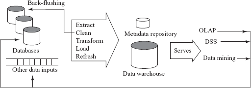
Fig. 14.1 A typical data warehouse architecture
Large companies have various data sources that have been constructed independently by different groups and likely to have different schemas. If the companies want to use such diverse data for making business decisions, they need to gather this data under a unified schema for efficient execution of queries. Moreover, there can be a number of semantic mismatches across these databases such as different currency units, different names for the same attribute, differences in the normalized forms of the tables, etc. These differences must be accommodated before the data is brought into the warehouse. Thus, the main task of data warehousing is to perform schema integration and to convert the data to an integrated schema before it is actually stored.
After the schema is designed, the warehouse must acquire data so that it can fulfil the required objectives. Acquisition of data for the warehouse involves the following steps:
- The data is extracted from multiple, heterogeneous data sources. The data sources include operational databases (databases of the organizations at various sites) and external sources such as web, purchased data, etc.
- The data sources may contain some minor errors or inconsistencies. For example, the names are often misspelled, and street, area or city names in the addresses are misspelled or zip codes are entered incorrectly. This incorrect data, thus, must be cleaned to minimize the errors and fill in the missing information when possible. The task of correcting and preprocessing the data is called data cleansing. These errors can be corrected to some reasonable level by looking up a database containing street names and zip codes in each city. The approximate matching of data required for this task is referred to as fuzzy lookup. In some cases, the data managers in the organization want to upgrade their data with the cleaned data. This process is known as back-flushing. This data is then transformed to accommodate semantic mismatches.
- The cleaned and transformed data is finally loaded into the warehouse. Data is partitioned, and indexes or other access paths are built for fast and efficient retrieval of data. Loading is a slow process due to the large volume of data. For instance, loading a terabyte of data sequentially can take weeks and a gigabyte can take hours. Thus, parallelism is important for loading warehouses. The raw data generated by transaction processing system may be too large to store in a data warehouse, therefore, some data can be stored in summarized form. Thus, additional preprocessing such as sorting and generation of summarized data is performed at this stage.
This entire process of getting data into the data warehouse is called extract, transform, and load (ETL) process. At the backend of the process, OLAP, data mining, and DSS may generate new relevant information such as rules and patterns. This information is sent back to the data warehouse. Once the data is loaded into a warehouse, it must be periodically refreshed to reflect the updates on the relations at the data sources and periodically purge old data. The updates of a warehouse are handled by the acquisition component of the warehouse that provides all required preprocessing.
Learn More
Microsoft’s SQL Server comes with a free ETL tool called Data Transforming Service (DTS).
The third and the most important component of the data warehouse is the metadata repository, which keeps track of currently stored data. It contains the description of the data including its schema definition. The metadata repository includes both technical and business metadata. The technical metadata includes the technical details of the warehouse including storage structures, data description, warehouse operations, etc. The business metadata, on the other hand, includes the relevant business rules of the organization.
14.1.2 Multidimensional Modeling for a Data Warehouse
The data in a warehouse is usually multidimensional data having measure attributes and dimension attributes. The attributes that measure some value and can be aggregated upon are called measure attributes. On the other hand, the attributes that define the dimensions on which the measure attributes and their summaries are viewed are called dimension attributes.
The relations containing such multidimensional data are called fact tables. The fact tables contain the primary information in the data warehouse, and thus are very large. Consider a bookshop selling books of different categories such as textbooks, language books, and novels, and it maintains an Online Book database for its customers so that they can buy books online. The bookshop may have several branches in different locations. The SALES relation shown in Figure 14.2 is an example of a fact table that stores the sales information of various books at different locations in different time periods. The attribute Number is the measure attribute, which describes the number of books sold.

Fig. 14.2 Dimension tables and fact tables
Each tuple in the SALES relation gives information about which book is sold, which location the book was sold from, and at what time the book was sold. Thus, book, location, and time are the dimensions of the sales and for a given book, location, and time, we have at most one associated sales value. Each dimension has a set of attributes associated with it. For example, the dimension time is identified by the attribute, tid in the SALES relation. Similarly, the dimensions book and location are identified by bid and lid, respectively. These identifiers are kept short in order to minimize the storage requirements.
The dimension attributes bid, tid, and lid in the fact tables are the primary keys in other tables called dimension tables (or lookup tables), which store additional information about the dimensions. For example, the book dimension can have the attributes Book_title, Category, and Price. Similarly, the location dimension can have the attributes City, State, Country. The time dimension can have the attributes Date, Week, Month, Quarter, and Year. This information about book, location, and time is stored in the dimension tables BOOK, LOCATION, and TIME, respectively, as shown in Figure 14.2. The attribute bid, tid, and lid are the primary keys in BOOK, TIME, and LOCATION table, respectively, and these attributes are the foreign keys in fact table SALES. The primary key of a fact table is usually a composite key that is made up of all its foreign keys. The dimension tables are much smaller than the fact table.
The set of values associated with each dimension can also be structured as a hierarchy. For example, the dimension time can be arranged in a hierarchy as shown in Figure 14.3(a). Dates belong to weeks and months, which are in turn contained in quarters, and quarters are contained in years. Similarly, a city belongs to a state and a state belongs to a country, which led to the location hierarchy as shown in Figure 14.3(b). In the same way, different books can belong to different categories, thereby, resulting in book hierarchy as shown in Figure 14.3(c).
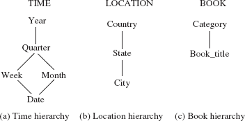
Fig. 14.3 Dimension hierarchies
The multidimensional data in a data warehouse can be represented either using a star schema or a snowflake schema. The star schema is the simplest data warehouse schema, which consists of a fact table with a single table for each dimension. The centre of the star schema consists of a large fact table and the points of the star are the dimension tables. The star schema for our running example is shown in Figure 14.4(a).
The snowflake schema is a variation of star schema, which may have multiple levels of dimension tables. For example, the attribute Book_title in BOOK relation can be a foreign key in another relation, say, BOOK_DETAILS with an additional attribute Descr that gives details of the book. Similarly, the attribute Quarter in the TIME relation can be a foreign key in another relation, say, QTR_DETAILS, with two additional attributes, Beg_date and End_date that give the starting and ending dates of each quarter, respectively. The snowflake schema for our running example is shown in Figure 14.4(b).
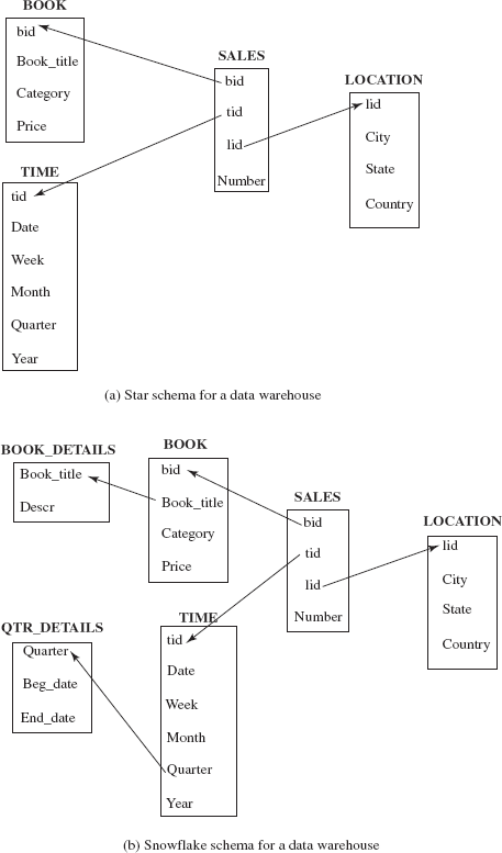
Fig. 14.4 Warehouse schemas
14.2 ONLINE ANALYTICAL PROCESSING (OLAP)
Online Analytical Processing (OLAP) is a category of software technology that enables analysts, managers, and executives to analyze the complex data derived from the data warehouse. The term online indicates that the analysts, managers, and executives must be able to request new summaries and get the responses online, within a few seconds. They should not be forced to wait for a long time to see the result of the query. OLAP enables data analysts to perform ad hoc analysis of data in multiple dimensions, thereby providing the insight and understanding they need for better decision-making.
NOTE SQL:1999 and SQL:2003 standards contain some additional constructs to support data analysis. The SQL extensions for data analysis are discussed in Appendix B.
Since the data in the data warehouse is multidimensional in nature, it may be difficult to analyze. Therefore, it can be displayed in the form of cross-tabulation as shown in Figure 14.5. A cross-tabulation (also known as a cross-tab or a pivot table) can be done on any two dimensions keeping the other dimensions fixed as all. In general, a cross-tab is a two-dimensional table in which values for one attribute (say A) form the row headers, and values for another attribute (say B) form the column headers. Each cell can be identified by (ai, bj) where ai is a value for A and bj is a value for B. If there is single tuple with any value, say (ai, bj), in the fact table, then the value in the cell is derived from that single tuple. However, if there are multiple tuples with (ai, bj) value, then the value in the cell is derived by aggregation on the tuples with that value. In most of the cases, an extra row and an extra column are used for storing the total of the cells in the row/column.

Fig. 14.5 Cross-tabulations of SALES relation
Figure 14.5(a) shows the cross-tabulation of SALES relation (shown in Figure 14.2) by bid and tid for all lid. Similarly, Figure 14.5(b) shows the cross-tabulation of SALES relation by lid and tid for all bid. Finally, Figure 14.5(c) shows the cross-tabulation of SALES relation by bid and lid for all tid.
Unlike relational tables where the number of columns is fixed, the number of columns in a cross-tab may change depending on the data stored in it. New columns can be added, and existing columns can be deleted depending on the data values. Thus, it is desirable to represent a cross-tab in the form of a relation with a fixed number of columns as shown in Figure 14.6. The summary values can be represented by introducing a special value, all, that represents subtotals. The SQL:1999 standard actually uses the null value in place of all. However, we have used all to avoid confusion with the null values stored in the database.
In the core of any OLAP system, there is a concept of a data cube (also called a multidimensional cube or OLAP cube or hypercube), which is the generalization of a 2D cross-tab to n dimensions. A three-dimensional data cube on the SALES relation is shown in Figure 14.7. In this figure, book dimension is shown on x-axis, time as y-axis, and location as z-axis. The value for a dimension may be all, in which case the cell contains a summary over all values of that dimension like a cross-tabulation.

Fig. 14.6 Relational representation of the cross-tab shown in figure 14.5(a)
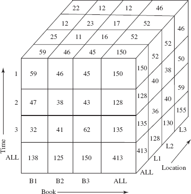
Fig. 14.7 Three-dimensional data cube for SALES relation
A data analyst can look at different cross-tabs on the same data by interactively selecting the dimensions in the cross-tab. The technique of changing from one-dimensional orientation to another is known as pivoting (or rotation). The pivoted version of the data cube in Figure 14.7 is shown in Figure 14.8. In this figure, book dimension is shown on x-axis, location as y-axis, and time as z-axis.
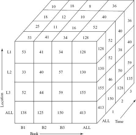
Fig. 14.8 Pivoted version of data cube shown in figure 14.7
In addition to pivoting, an OLAP system also provides some other functionalities, which are given as follows:
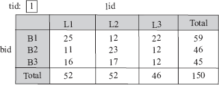
- Slice and dice: The data cube is full of data, and there are many thousands of combinations in which it can be viewed. In case a cross-tabulation is done for a specific value other than all for the fixed third dimension, it is called slice operation or slicing. Slicing can be thought of as viewing a slice of the data cube. For example, an analyst may want to see a cross-tab of
SALESrelation on the attributesbidandlidfortid=1, instead of the sum across all time periods. The resultant cross-tab is shown in Figure 14.9, which can be thought of as a slice orthogonal totidaxis. Slicing is sometimes called dicing when two or more dimensions are fixed. Slice and dice operations enable users to see the information that is most meaningful to them and examine it from different viewpoints.Note that instead of specifying all for the attributes that are not part of cross-tab, slicing/dicing consists of selecting specific values for these attributes, and displaying them on the top of the cross-tab. For example, in Figure 14.9,
tid=1is displayed on the top of the cross-tab instead of all.Fig. 14.9 Slicing the cube for
tid=1 - Rollup and drill down: OLAP system also allows data to be displayed at various levels of granularity. The operation that converts data with a finer-granularity to the coarser-granularity with the help of aggregation is known as rollup operation. On the other hand, an operation that converts data with a coarser-granularity to the finer-granularity is known as drill down operation. For example, an analyst may be interested in viewing the sales of books category wise (textbooks, language books, and novels) in different countries, instead of looking at individual sales. This is rollup operation. On the other hand, the analyst looking at the level of books categories may drill down the hierarchy to look at individual sales in different states of each country. The resultant cross-tabs after rollup and drill down operations on
SALESrelation are shown in Figure 14.10. The values are derived from the fact and dimension tables shown in Figure 14.2.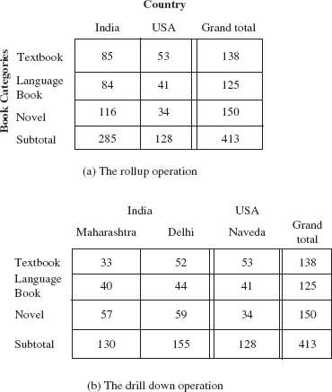
Fig. 14.10 Applying rollup and drill down operations on
SALESrelation
14.2.1 Implementing OLAP
There are three ways of implementing OLAP system. The traditional OLAP systems used multidimensional arrays in memory to store data cubes and thus, are referred to as multidimensional OLAP (MOLAP) systems. The OLAP systems that work directly with relational databases are called relational OLAP (ROLAP) systems. In ROLAP systems, the fact tables and dimension tables are stored as relations and new relations are also created to store the aggregated information.
MOLAP systems generally use specialized indexing and storage optimizations and hence, deliver better performance. MOLAP also needs less storage space compared to ROLAP, because the specialized storage typically includes compression techniques. Moreover, ROLAP relies more on the database to perform calculations, thus, it has more limitations in the specialized functions it can use. However, ROLAP is generally more scalable.
The systems that include the best of ROLAP and MOLAP are known as hybrid OLAP (HOLAP). These systems use main memory to hold some summaries, and relational tables to hold base data and other summaries. Therefore, it can generally pre-process quickly, scale well, and offer good function support.
Most of the OLAP systems are implemented as client/server systems. The client systems requests different views of the data from the server, which contains the relational database as well as MOLAP data cubes. The entire data cubes on a relation can be computed by using any standard algorithm for computing aggregate operations, one grouping at a time. However, this algorithm is the naive way to compute the data cube, as it may require scanning a relation large number of times.
A simple way to optimize the algorithm is to compute an aggregate from another aggregate, instead of from the base relation. A further improvement can be achieved by computing multiple groupings on a single scan of the data. Early OLAP implementations pre-computed and stored entire data cubes (groupings on all subsets of dimension attributes). The pre-computation allows OLAP queries to be answered within a few seconds, even if the database contains a large number of tuples.
However, the entire data cube is often larger than the original relation from which the data cube is formed, as there are 2n groupings for n dimension attributes. The number of groupings further increases with hierarchies on attributes. Thus, in most of the cases it is not feasible to store the entire data cubes. Instead of pre-computing and storing all the possible groupings, some of the groupings can be computed and stored, and others can be computed on demand. For example, consider a query that requires summaries by (bid, tid) which has not been pre-computed. The result can be computed from the summaries by (bid, tid, lid), if that has been already computed.
14.3 DATA MINING TECHNOLOGY
With rapid computerization in the past two decades, almost all the organizations have collected a vast amount of data in their databases. These organizations need to understand their data and also want to discover useful information in terms of patterns or rules from the existing data. The extraction of hidden and predictive information from such large databases is known as data mining. Data mining tools predict future trends and behaviours, which allow organizations to make proactive and knowledge-driven decisions. Identifying the profile of customers with similar buying habits, finding all items that are frequently purchased with some other item, finding all credit card applicants with poor or good credit risks are some of the examples of data mining queries.
Things to Remember
Data mining combines work from areas such as statistics, machine learning, pattern recognition, databases, and more recently high performance computing. The goal of data mining is to discover interesting and previously unknown information in the data sets. Tools for data mining have the ability to analyze enormous amount of data and discover significant patterns and relationships that might otherwise have taken a person thousand of hours to find.
Though data in large operational databases and flat files can be provided as input for the data mining process, data in data warehouses is more suitable for data mining process. Some of the advantages of using data of data warehouses for data mining are listed here.
- A data warehouse consists of data from multiple sources. Thus, the data in data warehouse is integrated and subject-oriented.
- In a data warehouse, the data is first extracted, cleaned, and transformed before loading, thus, maintaining the consistency of the data.
- The data in a data warehouse is in summarized form. Hence, the data mining process can directly use this data without performing any aggregations.
- A data warehouse also provides the capability of analysing the data by using OLAP operations.
14.3.1 Knowledge Discovery in Databases
Like knowledge discovery in artificial intelligence (also known as machine learning) or exploratory data analysis in statistics, data mining also tries to find useful patterns or rules from the data. However, it differs from machine learning and statistical analysis in a way that it deals with a large volume of data typically stored on disks. That is, data mining deals with knowledge discovery in databases (KDD). Knowledge discovery in databases is the non-trivial extraction of implicit, previously unknown, and potentially useful information from the databases. The process of KDD is divided into six phases that are given as follows:
- Data selection or extraction: The entire raw dataset is examined to identify the target subset of data and the attributes of interest.
- Data cleansing or preprocessing: The data is cleaned to minimize errors and fill in missing information, wherever possible.
- Enrichment: The data is enhanced with additional sources of information.
- Data transformation or encoding: The data is categorized under different groups in terms of categories, ranges, geographical regions, and so on. This may be done to reduce the amount of data stored in the database.
- Data mining: The data mining is applied to discover useful patterns and rules.
- Interpretation or evaluation: The patterns are presented to the users in easily understandable and meaningful formats such as listings, graphical outputs, summary tables or visualizations.
14.3.2 Types of Knowledge Discovered During Data Mining
The knowledge discovered from the database during data mining includes the following:
- Association rules: Association describes a relationship between a set of items that people tend to buy together. For example, if customers buy two-wheelers, there is a possibility that they also buy some accessories such as seat cover, helmet, gloves, etc. A good salesman, therefore, exploits them to make additional sales. However, our main aim is to automate the process so that the system itself may suggest accessories that tend to be bought along with two-wheelers. The association rules derived during data mining correlate a set of items with another set of items that do not intersect.
- Classification: The goal of classification is to partition the given data into predefined disjoint groups or classes. For example, an insurance company can define the insurance worthiness level of a customer as excellent, good, average or bad depending on the income, age, and prior claims experience of the customers.
- Clustering: The task of clustering is to group the data into set of similar elements so that those similar elements belong to the same class. The principle of clustering is to maximize intra-class similarity and minimize the inter-class similarity.
Association Rules
Discovery of association rules is one of the major tasks involved in data mining. The task of mining association rules is to find interesting relationship among various items in a given data set. Retail shops are generally interested in association between different items that customers buy. A common application is that of market-basket data where market-basket describes a set of items a consumer buys in a supermarket during his one visit. Consider some examples of associations given as follows:
- A person who buys a mobile is also likely to buy some accessories such as mobile cover, hands free, etc.
- A person who buys bread is also likely to buy butter and jam.
- Someone who buys eggs is also likely to buy bread.
- Someone who bought the book Data Structure using C is also likely to buy Programming in C.
The association information can be used in several ways. For example, a mobile shop may decide to keep attractive mobile covers to tempt people to buy them. Similarly, if a customer buys a book online, the system may also suggest associated books. A grocery shop may decide to place bread close to eggs, since they are often bought together. This will help the owners of retail shop, bookshop, and grocery shop to increase the sales of associated items.
An association rule has a form X⇒Y, where X={x1, x2, …, xn} and Y={y1, y2,…,yn} are the disjoint sets of items, that is, X∩Y=Ø. It states that if a person buys an item X, he or she is likely to buy an item Y. The set X∪Y is called an itemset—a set of items a customer tends to buy together. The item X is called the antecedent, while Y is called the consequent of the rule. An example of association rule is
mobile ⇒ mobile cover, hands free
This rule says that a customer who buys a mobile also tends to buy mobile cover and hands free. An association rule must have an associated population, which consists of a set of instances. For example, in a bookshop, the population may consist of all customers who made purchases regardless of when they made the purchases. Thus, each customer is an instance. However, in case of grocery shop, the population may consist of all grocery shop purchases irrespective of the number of visits of a single customer. Thus, each purchase (not a customer) is an instance. For an association rule to be of interest to an analyst, the rule should satisfy two interest measures, namely, support and confidence.
- Support (also known as prevalence): It is the percentage or fraction of a population that satisfies both the antecedent and consequent of the rule. If the support is low, it implies that there is no strong evidence that the items in the itemset
X∪Yare bought together. For example, suppose only 0.002% of the customers buy mobile and chocolates; thus, the support for the rule mobile ⇒ chocolates is low. Companies are generally not interested in such rules since they involve only a few customers. However, if 60% of the purchases involve mobile, mobile cover, and hands free, this implies that its support is high. Companies pay a lot of attention to the rules with high support. - Confidence (also known as strength): It is the probability that a customer will buy the items in the set
Yif he or she purchases the items in the setX. It is computed assupport(X∪Y)/support(X)
For example, the association rule mobile ⇒ mobile cover has the confidence of 80% if 80% of the purchases that include mobile also include mobile cover. Like a rule with low support, a rule with low confidence is also not meaningful for the organizations.
To understand the concept of support and confidence, consider some transactions of a mobile shop shown in Table 14.2. Let us consider two association rules, mobile ⇒ mobile cover and mobile ⇒ hands free. The support for mobile ⇒ mobile cover is 50% and the support for mobile ⇒ hands free is 75%. The confidence for mobile ⇒ mobile cover is 66.67%. It implies that out of three transactions, which contain mobile, two contain mobile cover. Further, the confidence for mobile ⇒ hands free is 100%. It implies that all the three transactions that contain mobile also contain hands free.
Table 14.2 Sample transactions in mobile shop
| Transaction_ID | Time | Items Purchased |
|---|---|---|
| T1 | 12:00 | Mobile, mobile cover, hands free |
| T5 | 2:00 | Mobile, hands free |
| T10 | 5:00 | Mobile, mobile cover, hands free, memory card |
| T20 | 8:00 | Hands free, memory card |
The main goal of mining association rules is to find all the possible rules that exceed some minimum prespecified support and confidence value. This problem of generating a set of possible association rules can be broken down in two sub-problems.
- Finding all itemsets that have support above the minimum prespecified support. These itemsets are called large (or frequent) itemsets.
- Deriving all rules for each large itemset, which have confidence more than the minimum prespecified confidence, and that involve all and only the elements of the set.
If there are n number of items in a company, then the number of distinct itemsets will be 2n and computing support for all possible itemsets becomes very tedious and time-consuming. To reduce the combinatorial search space, algorithms for finding association rules make use of these properties.
- Downward closure: This property states that each subset of a large itemset must also be large.
- Anti-monotonicity: This property states that each superset of a small itemset is also small. Thus, once an itemset is found to have small support, any extensions formed by adding one or more items to the set will also produce a small subset.
There are several algorithms to find the large itemsets. One of them is Apriori algorithm.
Apriori Algorithm Apriori algorithm uses the downward closure property. It takes a database D of t transactions and minimum support, minSup, represented as a fraction of t, as input. Apriori algorithm generates all possible large itemsets L1, L2, …, Lk as output. The algorithm is shown in Figure 14.11.
The algorithm proceeds iteratively. In the first pass, only the sets with single items are considered for generating large itemsets. This itemset is referred to as large 1-itemset (itemset with one item). In each subsequent pass, large itemsets identified in the previous pass are extended with another item to generate larger itemsets. Therefore, the second pass considers only sets with two items, and so on. Thus, by considering only the itemsets obtained by extending the large itemsets, we reduce the number of candidate large itemsets. The algorithm terminates after k passes, if no large k -itemsets is found.
  Step 1: k=1;
  Step 2: Find large itemset Lk from Ck; //Ck is the set of all
                                        //candidate itemsets
  Step 3: Form Ck+1 from Lk;
  Step 4: k=k+1;
  Step 5: Repeat steps 2, 3, and 4 until Ck is empty;
Fig. 14.11 Apriori algorithm
Step 2 is called the large itemset generation step, and step 3 is called the candidate itemset generation step. The details about steps 2 and 3 are explained in Figure 14.12.
Step 2: Large itemset generation
    Step 2a: Scan the database D and count each itemset in Ck;
    Step 2b: If the count is greater than minSup then
                     add that itemset to Lk;
Step 3: Candidate itemset generation
    Step 3a: For k=1, C1 = all itemsets of length 1;
             For k>1, generate Ck from Lk–1 as follows:
            The join step:
                 Ck = k–2 way join of Lk–1 with itself;
                 If both {I1,.., Ik–2, Ik-1} and {I1,.., Ik–2, Ik} are in Lk–1 then add {I1,..,Ik–2, Ik–1, Ik} to Ck;
//assuming that the items I1,…,Ik are always sorted
The prune step:
Remove {I1, …,Ik–2, Ik–1, Ik}, if it does not contain a large (k–1)subset;
Fig. 14.12 Details of steps 2 and 3 of apriori algorithm
An example of Apriori algorithm is shown in Figure 14.13. Let the value of minSup be 50%, that is, the item in the candidate set should be included in at least two transactions. In the first pass, the database D is scanned to find the candidate itemset C1 from which large 1-itemset L1 is produced. Since the support for itemset {4} is less than the minSup, it is not included in L1. In the second pass, candidate itemset C2 is generated from L1, which consists of {1,2}, {1,3}, {1,5}, {2,3}, {2,5}, and {3,5}. Then the database D is scanned to find the support for these itemsets and produce large 2-itemsets L2. Since the support for itemsets {1, 2} and {1, 5} is less than the minSup, they are not included in L2. In the third pass, candidate itemset C3 is generated from L2, which includes {2,3,5}. The database D is again scanned to find the support for this itemset and produce large 3-itemsets L3, which is the desired large itemset.

Fig. 14.13 An example of apriori algorithm
Once the large itemsets are identified, the next step is to generate all possible association rules. Association rules can be found from every large itemset L with the help of another algorithm shown in Figure 14.14.
    For every non-empty subset S of L
    Find B = L–A.
    A⇒B is an association rule if
         confidence(A⇒B)>=minConf
                    //confidence(A⇒B)=support(A∪B)/support(A)
Fig. 14.14 An algorithm for finding association rules
For example, consider the large itemset L = {2, 3, 5} generated earlier with support 50%. Proper non-empty subsets of L are: {2, 3}, {2, 5}, {3, 5}, {2}, {3}, {5} with supports = 50%, 75%, 50%, 75%, 75%, and 75%, respectively. The association rules from these subsets are given in Table 14.3.
Table 14.3 A set of association rules
| Association Rule A⇒B | Confidence Support(A∪B)/Support(A) |
|---|---|
| {2, 3} ⇒ {5} | 50% / 50% = 100% |
| {2, 5} ⇒ {3} | 50% / 75% = 66.67% |
| {3, 5} ⇒ {2} | 50% / 50% = 100% |
| {2} ⇒ {3, 5} | 50% / 75% = 66.67% |
| {3} ⇒ {2, 5} | 50% / 75% = 66.67% |
| {5} ⇒ {2, 3} | 50% / 75% = 66.67% |
Classification
Classification can be done by finding rules that partition the given data into predefined disjoint groups or classes. The task of classification is to predict the class of a new item; given that items belong to one of the classes, and given past instances (known as training instances) of items along with the classes to which they belong. The process of building a classifier starts by evaluating the training data (or training set), which is basically the old data that has already been classified by using the domain of the experts’ knowledge.
For example, consider an insurance company that wants to decide whether or not to provide insurance facility to a new customer. The company maintains records of its existing customers, which may include name, address, gender, income, age, types of policies purchased, and prior claims experience. Some of this information may be used by the insurance company to define the insurance worthiness level of the new customers. For instance, the company may assign the insurance worthiness level of excellent, good, average, or bad to its customers depending on the prior claims experience.
Note that new customers cannot be classified on the basis of prior claims experience as this information is unavailable for new customers. Therefore, the company attempts to find some rules that classify its current customers on the basis of the attributes other than the prior claim experience. Consider four such rules that are based on two attributes, age and income.
Rule 1: ∀customer C, C.age<30 and C.income<=30,000 ⇒ C.insurance=bad
Rule 2: ∀customer C, C.age≥30 and C.age<50 and C.income>75,000 ⇒ C.insurance=excellent
Rule 3: ∀customer C, (C.age≥50 and C.age≤60) and (C.income≥30,000 and C.income≤75,000) ∀ C.insurance=good
Rule 4: ∀customer C, C.age>60 and C.income>30,000 ⇒ C.insurance=average
This type of activity is known as supervised learning since the partitions are done on the basis of the training instances that are already partitioned into predefined classes. The actual data, or the population, may consist of all new and the existing customers of the company. There are several techniques used for classification. One of them is decision tree classification.
Decision Tree Classification A decision tree (also known as a classification tree) is a graphical representation of the classification rules. Each internal node of the decision tree is labelled with an attribute Ai. Each arc is labelled with the predicate (or condition), which can be applied to the attribute at the parent node. Each leaf node is labelled with one of the predefined classes. Therefore, each internal node is associated with a predicate and each leaf node is associated with a class. An example of decision tree is shown in Figure 14.15.

Fig. 14.15 An example of a decision tree
Given a set of training data, the question is how to build a decision tree. There are many algorithms to construct a decision tree. The most commonly used algorithm searches through the attributes of the training set and extracts the attribute that best separates the given instances. This attribute is called the partitioning attribute. If the partitioning attribute A perfectly classifies the training sets, the algorithm stops, otherwise it recursively selects partitioning attribute and partitioning predicate to create further child nodes. The algorithm uses a greedy search, that is, it picks the best attribute and never looks back to reconsider earlier choices.
In Figure 14.15, the attribute age is chosen as a partitioning attribute, and four child nodes—one for each partitioning predicate 0–30, 30–50, 50–60, and over 60—are created. For all these child nodes, the attribute income is chosen to further partition the training instances belonging to each child node. Depending on the value of the income, a class is associated with customer. For example, if the age of the customer is between 50 and 60, and his income is greater than Rs 75,000, then the class associated with him is ‘excellent’.
Clustering
The process of grouping the records together so that the degree of association is strong between the records of the same group and weak between the records of different groups is known as clustering. Unlike classification, clustering is unsupervised learning as no training sample is available to guide partitioning. The groups created in this case are also disjoint. Grouping of customers on the basis of similar buying patterns, grouping of students in a class on the basis of grades (A, B, C, D, E or F), etc., are some of the common examples of clustering.
The quality of clustering result depends on the similarity measure. A similarity function based on the distance is typically used if the data is numeric. For example, the Euclidean distance can be used to measure similarity. The Euclidean distance between two n-dimensional records (records with n attributes) ri and rj can be computed as follows:
The smaller the distance between two records, the greater is the similarity between them. The most commonly used algorithm used for clustering is k-means algorithm, where k is the number of desired clusters, as shown in Figure 14.16.
Input: a set of m records r1, …, rm and number of desired clusters k
Output: set of k clusters
Process:
     Step 1: Start
     Step 2: Randomly choose k records as the centroid (mean) for k clusters;
     Step 3: Repeat steps 4 and 5 until no change
     Step 4: For each record ri, find the distance of the record from the centroid of each cluster and assign that record to the cluster from which it has the
     Step 5: Recompute the centroid for each cluster based on the current records present in the cluster;
     Step 6: Stop minimum distance;
Fig. 14.16 k-means algorithm for clustering
Let us understand the algorithm with the help of an example. Consider a sample of 2D records shown in Table 14.4. Assume that the number of desired clusters k = 2. The centroid (mean) of a cluster Ci containing m n -dimensional records can be calculated as follows:

Table 14.4 Sample 2D data for clustering
| Age | Income (,000) |
|---|---|
| 20 | 10 |
| 30 | 20 |
| 30 | 30 |
| 35 | 35 |
| 40 | 40 |
| 50 | 45 |
Step 1: Let the algorithm randomly choose record 2 for cluster C1 and record 5 for cluster C2. Thus, the centroid for C1 is (30, 20) and C2 is (40, 40).
Step 2: Calculate the distance of the remaining records from the centroid of both C1 and C2, and assign the record to the cluster from which it has the minimum distance as shown in Table 14.5.
Table 14.5 Distance of records from centroids of C1 and C2

Now, records 1 and 2 are assigned to cluster C1 and records 3, 4, 5, and 6 are assigned to cluster C2.
Step 3: Recompute the centroid of both the clusters. The new centroid for C1 is (25, 15) and for C2 is (38.75, 37.5). Again calculate the distance of all six records from the new centroid and assign the records to the appropriate cluster as shown in Table 14.6.
Table 14.6 Distance of all six records from new centroids of C1 and C2
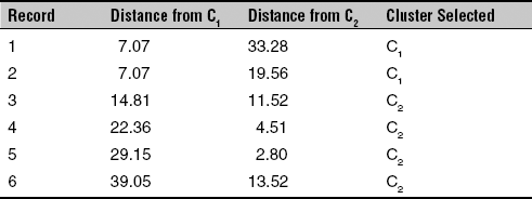
After the step 3, the records 1 and 2 are assigned to cluster C1 and records 3, 4, 5, and 6 are assigned to cluster C2. Since after step 3, the records remain in the same cluster as they were in step 2, the algorithm terminates after this step.
14.3.3 Application Areas of Data Mining
Data mining can be used in many areas such as banking, finance, and telecommunications industries. Some of the significant applications of data mining technologies are given here.
- Market-basket analysis: Companies can analyse the customer behaviour based on their buying patterns, and may launch products according to the customer needs. The companies can also decide their marketing strategies such as advertising, store location, etc. They can also segment their customers, stores or products based on the data discovered after data mining.
- Investment analysis: Customers can also look at the areas such as stocks, bonds, and mutual funds where they can invest their money to get good returns.
- Fraud detection: By finding the association between frauds, new frauds can be detected using data mining.
- Manufacturing: Companies can optimize their resources like machines, manpower, and materials by applying data mining technologies.
- Credit risk analysis: Given a set of customers and an assessment of their credit worthiness, descriptions for various classes can be developed. These descriptions can be used to classify a new customer into one of the classes.
Other than these significant areas, some other applications of data mining include quality control, process control, medical management, store management, student recruitment and retention, pharmaceutical research, electronic commerce, claims processing, and so on. The full spectrum of application areas is very broad.
SUMMARY
- The database applications that record and update data about transactions are known as online transaction processing (OLTP) applications.
- The systems that aim to extract high-level information stored in OLTP databases, and to use that information in making a variety of decisions that are important for the organization are known as decision-support systems (DSS).
- Several tools and techniques are available that provide the correct level of information to help the decision makers in decision-making. Some of these tools and techniques include data warehousing, online analytical processing (OLAP), and data mining.
- A data warehouse (DW) is a repository of suitable operational data (data that documents the everyday operations of an organization) gathered from multiple sources, stored under a unified schema, at a single site.
- According to William Inmon, the father of the modern data warehouse, a data warehouse is a subject-oriented, integrated, time-variant, non-volatile collection of data in support of management’s decisions.
- The main advantage of using a data warehouse is that a data analyst can perform complex queries and analyses on the information stored in data warehouse without affecting the OLTP systems.
- A data warehouse basically consists of three components, namely, the data sources, the ETL, and the schema of data stored in data warehouse including the metadata.
- While creating a data warehouse, the data is extracted from multiple, heterogeneous data sources. Then data cleansing is performed to remove any kind of minor errors and inconsistencies. This data is then transformed to accommodate semantic mismatches. The cleaned and transformed data is finally loaded into the warehouse.
- The entire process of getting data into the data warehouse is called extract, transform, and load (ETL) process.
- The third and the most important component of the data warehouse is the metadata repository, which keeps track of currently stored data. It contains the description of the data including its schema definition.
- The data in a warehouse is usually multidimensional data having measure attributes and dimension attributes.
- The attributes that measure some value and can be aggregated upon are called measure attributes. On the other hand, the attributes that define the dimensions on which the measure attributes and their summaries are viewed are called dimension attributes.
- The relations containing such multidimensional data are called fact tables. The dimension attributes in the fact tables are the primary keys in other tables called dimension tables, which store additional information about the dimensions.
- The multidimensional data in a data warehouse can be represented either using a star schema or a snowflake schema.
- The star schema is the simplest data warehouse schema, which consists of a fact table with a single table for each dimension. The snowflake schema is a variation of star schema, which may have multiple levels of dimension tables.
- Online Analytical Processing (OLAP) is a category of software technology that enables analysts, managers, and executives to analyse the complex data derived from the data warehouse.
- Since the data in the data warehouse is multidimensional in nature, it may be difficult to analyse. Therefore, it can be displayed in the form of cross-tabulation.
- A cross-tab is a two-dimensional table in which values for one attribute (say
A) form the row headers, and values for another attribute (sayB) form the column headers. Each cell in the cross-tab can be identified by (ai,bj), whereaiis a value forAandbjis a value forB. - A data cube (also called a multidimensional cube or OLAP cube or hypercube) is the generalization of a two-dimensional cross-tab to n dimensions.
- A data analyst can look at different cross-tabs on the same data by interactively selecting the dimensions in the cross-tab. The technique of changing from one-dimensional orientation to another is known as pivoting (or rotation).
- In case a cross-tabulation is done for a specific value other than all for the fixed third dimension, it is called slice operation or slicing. Slicing is sometimes called dicing when two or more dimensions are fixed.
- The operation that converts data with a finer-granularity to the coarser-granularity with the help of aggregation is known as rollup operation. An operation that converts data with a coarser-granularity to the finer-granularity is known as drill down operation.
- There are three ways of implementing OLAP system. The traditional OLAP systems use multidimensional arrays in memory to store data cubes and thus, are referred to as multidimensional OLAP (MOLAP) systems.
- The OLAP systems that work directly with relational databases are called relational OLAP (ROLAP) systems.
- The systems that include the best of ROLAP and MOLAP are known as hybrid OLAP (HOLAP) systems. These systems use main memory to hold some summaries, and relational tables to hold base data and other summaries.
- The extraction of hidden and predictive information from a vast amount of data is known as data mining.
- Data mining deals with knowledge discovery in databases (KDD). KDD is the non-trivial extraction of implicit, previously unknown, and potentially useful information from the databases.
- The knowledge discovered from the database during data mining includes association rules, classification, and clustering.
- The task of mining association rules is to find interesting relationship among various items in a given data set.
- An association rule must have an associated population, which consists of a set of instances.
- For an association rule to be of interest to an analyst, the rule should satisfy two interest measures, namely, support and confidence.
- The itemsets that have support above the minimum prespecified support are known as large (or frequent) itemsets.
- The task of classification is to predict the class of a new item given that items belong to one of the classes, and given past instances (known as training instances) of items along with the classes to which they belong.
- A decision tree (also known as classification tree) is a graphical representation of the classification rules.
- The process of grouping the records together so that the degree of association is strong between the records of the same group and weak between the records of different groups is known as clustering.
- Online transaction processing (OLTP) system
- Decision-support system (DSS)
- Data warehouse
- Data mart
- Data extraction
- Data cleansing
- Fuzzy lookup
- Back-flushing
- Extract, transform and load (ETL) process
- Metadata repository
- Technical metadata
- Business metadata
- Multidimensional data
- Measure attributes
- Dimension attributes
- Fact table
- Dimension table (lookup table)
- Star schema
- Snowflake schema
- Online analytical processing (OLAP)
- Pivot table (cross-tab)
- Data cube (OLAP cube)
- Pivoting (rotation)
- Slicing and dicing
- Rollup and drill down operation
- Multidimensional OLAP (MOLAP)
- Relational OLAP (ROLAP)
- Hybrid OLAP (HOLAP)
- Data mining
- Knowledge discovery in database (KDD)
- Association rules
- Itemset
- Antecedent
- Consequent
- Population
- Instances
- Support (prevalence)
- Confidence (strength)
- Large (frequent) itemset
- Downward closure
- Anti-monotonicity
- Apriori algorithm
- Classification
- Training instances
- Training data (training set)
- Supervised learning
- Decision tree (classification tree)
- Greedy search
- Clustering
- Unsupervised learning
- k-means algorithm
EXERCISES
A. Multiple Choice Questions
- Which of the following is not a basic characteristic of a data warehouse?
- Subject oriented
- Volatile
- Time varying
- Integrated
- Which of the following statements is incorrect for a data warehouse?
- Which of the following is a basic component of a data warehouse?
- Data sources
- ETL process
- Metadata repository
- All of these
- Which of the following tables contain the primary information in the data warehouse?
- Primary table
- Dimension table
- Fact table
- Lookup table
- The technique of changing from one-dimensional orientation to another is known as _____________.
- Pivoting
- Slicing
- Dicing
- Drill down
- Which of the following OLAP systems work directly with relational databases?
- HOLAP
- ROLAP
- MOLAP
- None of these
- Which of the following is not a part of the KDD process?
- Data selection
- Data cleansing
- Enrichment
- Data warehousing
- The percentage or fraction of the population that satisfies both the antecedent and consequent of the rule is known as ______________.
- Support
- Population
- Confidence
- Instance
- Which of the following techniques is used for classification during data mining?
- Apriori algorithm
- k-means algorithm
- Decision tree
- Any of these
- Which of the following is an application area of data mining?
- Market-basket analysis
- Fraud detection
- Investment analysis
- All of these
B. Fill in the Blanks
- A _______________ is a repository of suitable operational data (data that documents the everyday operations of an organization) gathered from multiple sources, stored under a unified schema, at a single site.
- This entire process of getting data into the data warehouse is called _______________ process.
- The _______________ contains the description of the data including its schema definition.
- The multidimensional data in a data warehouse can be represented either using a ___________ or a ____________.
- ____________________ is a category of software technology that enables analysts, managers, and executives to analyse the complex data derived from the data warehouse.
- A ____________ is the generalization of a two-dimensional cross-tab to n dimensions.
- The operation that converts data with a finer-granularity to the coarser-granularity with the help of aggregation is known as ____________ operation.
- The extraction of hidden and predictive information from such large databases is known as _____________.
- ___________ describes a relationship between a set of items that people tend to buy together.
- The ______________ is basically the old data that has already been classified by using the domain of the experts’ knowledge.
C. Answer the Questions
- What are decision-support systems? What are the various tools and techniques that support decision-making activities?
- What is a data warehouse? How does it differ from an OLTP system?
- Define the following terms:
- ETL process
- Fuzzy lookup
- Data cube
- HOLAP
- Frequent itemsets
- Downward closure and anti-monotonicity
- Discuss the four basic characteristics of a data warehouse. What are the advantages of using a data warehouse?
- Describe the steps of building a data warehouse.
- What is role of the metadata repository in a data warehouse?
- What are dimension and measure attributes in the multidimensional data model?
- What is a fact table? How does it differ from a dimension table?
- Differentiate between a star schema and snowflake schema representation of a data warehouse.
- What is OLAP? What are the various ways of implementing OLAP? What is the basic difference between MOLAP and ROLAP?
- What is a pivot table? How does it help in analysing multidimensional data? Explain with the help of an example.
- Discuss the various functionalities that an OLAP system provides to analyze the data. Explain with the help of suitable examples.
- What is data mining? How is it different from knowledge discovery in artificial intelligence?
- ‘Though data in large operational databases and flat files can be provided as input for the data mining process, data in data warehouses is more suitable for data mining process.’ Why?
- What is KDD? Discuss the different phases of KDD process.
- What are association rules in the context of data mining? Describe the terms support and confidence with the help of suitable examples.
- Discuss the Apriori algorithm for generating large itemsets. Apply this algorithm for generating large itemset on the following dataset:
Transaction_ID Items Purchased T101 I1, I3, I4 T200 I2, I3, I5 T550 I1, I2, I3, I5 T650 I2, I5 - What is classification in context of data mining? Why is it called supervised learning? How is classification different from clustering?
- Discuss the k-means algorithm for clustering with the help of an example.
- What are the various applications of data mining?