
Chapter 1
The Fundamentals
1.1 Electrical Fundamentals
This chapter has been designed to provide you with the background knowledge required to help you understand the concepts introduced in the later chapters. If you have studied electrical science, electrical principles, or electronics then you will already be familiar with many of these concepts. If, on the other hand, you are returning to study or are a newcomer to electronics or electrical technology this chapter will help you get up to speed.
1.1.1 Fundamental Units
You will already know that the units that we now use to describe such things as length, mass and time are standardized within the International System of Units (SI). This SI system is based upon the seven fundamental units (see Table 1.1).
Table 1.1 SI units
| Quantity | Unit | Abbreviation |
| Current | ampere | A |
| Length | meter | m |
| Luminous intensity | candela | cd |
| Mass | kilogram | kg |
| Temperature | Kelvin | K |
| Time | second | s |
| Matter | mol | mol |
1.1.2 Derived Units
All other units are derived from these seven fundamental units. These derived units generally have their own names and those commonly encountered in electrical circuits are summarized in Table 1.2, together with the corresponding physical quantities.
Table 1.2 Electrical quantities

(Note that 0K is equal to −273°C and an interval of 1K is the same as an interval of 1°C.)
If you find the exponent notation shown in Table 1.2 a little confusing, just remember that V−1 is simply 1/V, s−1 is 1/s, m−2 is 1/m−2, and so on.
Example 1.1
The unit of flux density (the tesla) is defined as the magnetic flux per unit area. Express this in terms of the fundamental units.
Solution
The SI unit of flux is the weber (Wb). Area is directly proportional to length squared and, expressed in terms of the fundamental SI units, this is square meters (m2). Dividing the flux (Wb) by the area (m2) gives Wb/m2 or Wb m−2. Hence, in terms of the fundamental SI units, the tesla is expressed in Wb m−2.
Example 1.2
The unit of electrical potential, the volt (V), is defined as the difference in potential between two points in a conductor, which when carrying a current of one amp (A), dissipates a power of one watt (W). Express the volt (V) in terms of joules (J) and coulombs (C).
Solution
In terms of the derived units:

Note that: Watts = Joules/seconds and also that Amperes × seconds = Coulombs.
Alternatively, in terms of the symbols used to denote the units:
![]()
One volt is equivalent to one joule per coulomb.
1.1.3 Measuring Angles
You might think it strange to be concerned with angles in electrical circuits. The reason is simply that, in analog and AC circuits, signals are based on repetitive waves (often sinusoidal in shape). We can refer to a point on such a wave in one of two basic ways, either in terms of the time from the start of the cycle or in terms of the angle (a cycle starts at 0° and finishes as 360°—see Figure 1.1). In practice, it is often more convenient to use angles rather than time; however, the two methods of measurement are interchangeable and it’s important to be able to work in either of these units.

Figure 1.1 One cycle of a sine wave voltage
In electrical circuits, angles are measured in either degrees or radians (both of which are strictly dimensionless units). You will doubtless already be familiar with angular measure in degrees where one complete circular revolution is equivalent to an angular change of 360°. The alternative method of measuring angles, the radian, is defined somewhat differently. It is the angle subtended at the center of a circle by an arc having length that is equal to the radius of the circle (see Figure 1.2).

Figure 1.2 Definition of the radian
You may sometimes find that you need to convert from radians to degrees, and vice versa. A complete circular revolution is equivalent to a rotation of 360° or 2π radians (note that π is approximately equal to 3.142). Thus, one radian is equivalent to 360/2π degrees (or approximately 57.3°). Try to remember the following rules that will help you to convert angles expressed in degrees to radians and vice versa:
Example 1.4
Express an angle of 215° in radians.
Solution
To convert from degrees to radians, divide by 57.3. So, 215° is equivalent to 215/57.3 = 3.75 radians.
Example 1.5
Express an angle of 2.5 radians in degrees.
Solution
To convert from radians to degrees, multiply by 57.3. Hence, 2.5 radians is equivalent to 2.5 × 57.3 = 143.25°.
1.1.4 Electrical Units and Symbols
Table 1.3 shows the units and symbols that are commonly encountered in electrical circuits. It is important to get to know these units and also be able to recognize their abbreviations and symbols. You will meet all of these units later in this chapter.
Table 1.3 Electrical units

1.1.5 Multiples and Sub-Multiples
Unfortunately, many of the derived units are either too large or too small for convenient everyday use, but we can make life a little easier by using a standard range of multiples and sub-multiples (see Table 1.4).
Table 1.4 Multiples and sub-multiples
| Prefix | Abbreviation | Multiplier |
| tera | T | 1012 (= 1,000,000,000,000) |
| giga | G | 109 (= 1,000,000,000) |
| mega | M | 106 (= 1,000,000) |
| kilo | K | 103 (= 1,000) |
| (none) | (none) | 100 (= 1) |
| centi | c | 10−2 (= 0.01) |
| milli | m | 10−3 (= 0.001) |
| micro | μ | 10−6 (= 0.000001) |
| nano | n | 10−9 (= 0.000000001) |
| pico | p | 10−12 (= 0.000000000001) |
Example 1.6
An indicator lamp requires a current of 0.075A. Express this in mA.
Solution
You can express the current in mA (rather than in A) by simply moving the decimal point three places to the right. Hence, 0.075A is the same as 75 mA.
Example 1.7
A medium-wave radio transmitter operates on a frequency of 1,495 kHz. Express its frequency in MHz.
Solution
To express the frequency in MHz rather than kHz, we need to move the decimal point three places to the left. Hence, 1,495 kHz is equivalent to 1.495 MHz.
Solution
To express the value in μF rather than pF we need to move the decimal point six places to the left. Hence, 27,000 pF is equivalent to 0.027 μF (note that we have had to introduce an extra zero before the 2 and after the decimal point).
1.1.6 Exponent Notation
Exponent notation (or scientific notation) is useful when dealing with either very small or very large quantities. It’s well worth getting to grips with this notation as it will allow you to simplify quantities before using them in formulae.
Exponents are based on powers of ten. To express a number in exponent notation the number is split into two parts. The first part is usually a number in the range 0.1 to 100 while the second part is a multiplier expressed as a power of ten.
For example, 251.7 can be expressed as 2.517 × 100, i.e., 2.517 × 10². It can also be expressed as 0.2517 × 1,000, i.e., 0.2517 × 10³. In both cases the exponent is the same as the number of noughts in the multiplier (i.e., 2 in the first case and 3 in the second case). To summarize:
![]()
As a further example, 0.01825 can be expressed as 1.825/100; that is, 1.825 × 10⁻². It can also be expressed as 18.25/1,000, i.e., 18.25 × 10⁻³. Again, the exponent is the same as the number of zeros but the minus sign is used to denote a fractional multiplier. To summarize:
![]()
1.1.7 Multiplication and Division Using Exponents
Exponent notation really comes into its own when values have to be multiplied or divided. When multiplying two values expressed using exponents, you simply need to add the exponents. Here’s an example:
![]()
Similarly, when dividing two values which are expressed using exponents, you only need to subtract the exponents. As an example:
![]()
In either case it’s important to remember to specify the units, multiples and sub-multiples in which you are working (e.g., A, kΩ, mV, μF, etc.).
Example 1.11
A current of 3 mA flows in a resistance of 33 kΩ. Determine the voltage dropped across the resistor.
Solution
Voltage is equal to current multiplied by resistance. Thus:
![]()
Expressing this using exponent notation gives:
![]()
Separating the exponents gives:
![]()
Thus, V = 99 × 10(−3+3) = 99 × 100 = 99 × 1 = 99V
Example 1.12
A current of 45 μA flows in a circuit. What charge is transferred in a time interval of 20 ms?
Solution
Charge is equal to current multiplied by time (see the definition of the ampere). Thus:
![]()
Expressing this in exponent notation gives:
![]()
Separating the exponents gives:
![]()
Thus, Q = 900 × 10(−6−3) = 900 × 10−9 = 900 nC
Example 1.13
A power of 300 mW is dissipated in a circuit when a voltage of 1,500V is applied. Determine the current supplied to the circuit.

1.1.8 Conductors and Insulators
Electric current is the name given to the flow of electrons (or negative charge carriers). Electrons orbit around the nucleus of atoms just as the earth orbits around the sun (see Figure 1.3). Electrons are held in one or more shells, constrained to their orbital paths by virtue of a force of attraction toward the nucleus, which contains an equal number of protons (positive charge carriers). Since like charges repel and unlike charges attract, negatively charged electrons are attracted to the positively charged nucleus. A similar principle can be demonstrated by observing the attraction between two permanent magnets; the two North u.c. Poles of the magnets will repel each other, while a North and South u.c. Pole will attract. In the same way, the unlike charges of the negative electron and the positive proton experience a force of mutual attraction.

Figure 1.3 A single atom of helium (He) showing its two electrons in orbit around its nucleus
The outer shell electrons of a conductor can be reasonably easily interchanged between adjacent atoms within the lattice of atoms of which the substance is composed. This makes it possible for the material to conduct electricity. Typical examples of conductors are metals such as copper, silver, iron and aluminum. By contrast, the outer shell electrons of an insulator are firmly bound to their parent atoms and virtually no interchange of electrons is possible. Typical examples of insulators are plastics, rubber, and ceramic materials.
1.1.9 Voltage and Resistance
The ability of an energy source (e.g., a battery) to produce a current within a conductor may be expressed in terms of electromotive force (e.m.f.). Whenever an e.m.f. is applied to a circuit a potential difference (p.d.), or voltage, exists. Both e.m.f. and p.d. are measured in volts (V). In many practical circuits there is only one e.m.f. present (the battery or supply), whereas a voltage will be developed across each component present in the circuit.
The conventional flow of current in a circuit is from the point of more positive potential to the point of greatest negative potential (note that electrons move in the opposite direction!). Direct current results from the application of a direct e.m.f. (derived from batteries or a DC power supply). An essential characteristic of these supplies is that the applied e.m.f. does not change its polarity (even though its value might be subject to some fluctuation).
For any conductor, the current flowing is directly proportional to the e.m.f. applied. The current flowing will also be dependent on the physical dimensions (length and cross-sectional area) and material of which the conductor is composed.
The amount of current that will flow in a conductor when a given e.m.f. is applied is inversely proportional to its resistance. Therefore, resistance may be thought of as an opposition to current flow; the higher the resistance the lower the current that will flow (assuming that the applied e.m.f. remains constant).
1.1.10 Ohm’s Law
Provided that temperature does not vary, the ratio of p.d. across the ends of a conductor to the current flowing in the conductor is a constant. This relationship is known as Ohm’s Law and it leads to the relationship:
![]()
where V is the potential difference (or voltage drop) in volts (V), I is the current in amperes (A), and R is the resistance in ohms (Ω) (see Figure 1.4).
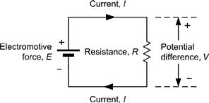
Figure 1.4 Simple circuit to illustrate the relationship between voltage (V), current (I) and resistance (R). Note that the direction of conventional current flow is from positive to negative.
The formula may be arranged to make V, I or R the subject, as follows:
![]()
The triangle shown in Figure 1.5 should help you remember these three important relationships. However, it’s worth noting that, when performing calculations of currents, voltages and resistances in practical circuits it is seldom necessary to work with an accuracy of better than ±1% simply because component tolerances are usually greater than this. Furthermore, in calculations involving Ohm’s Law, it can sometimes be convenient to work in units of kΩ and mA (or MΩ and μA) in which case potential differences will be expressed directly in V.

Figure 1.5 Triangle showing the relationship between V, I and R
Solution
Here we must use I = V/R (where V = 6V and R = 12Ω):
![]()
Hence a current of 500 mA will flow in the resistor.
Example 1.15
A current of 100 mA flows in a 56Ω resistor. What voltage drop (potential difference) will be developed across the resistor?
Solution
Here we must use V = I × R and ensure that we work in units of volts (V), amperes (A), and ohms (Ω).
![]()
(Note that 100 mA is the same as 0.1A.)
This calculation shows that a p.d. of 5.6V will be developed across the resistor.
Example 1.16
A voltage drop of 15V appears across a resistor in which a current of 1 mA flows. What is the value of the resistance?
Solution
![]()
Note that it is often more convenient to work in units of mA and V, which will produce an answer directly in kΩ, that is:
![]()
1.1.11 Resistance and Resistivity
The resistance of a metallic conductor is directly proportional to its length and inversely proportional to its area. The resistance is also directly proportional to its resistivity (or specific resistance). Resistivity is defined as the resistance measured between the opposite faces of a cube having sides of 1 cm.
The resistance, R, of a conductor is given by the formula:
![]()
where R is the resistance (ft), ρ is the resistivity (Ωm), l is the length (m), and A is the area (m2).
Table 1.5 shows the electrical properties of some common metals.
Table 1.5 Properties of some common metals

Example 1.17
A coil consists of an 8m length of annealed copper wire having a cross-sectional area of 1 mm2. Determine the resistance of the coil.
Solution
We will use the formula, R = ρ l/A.
The value of ρ for annealed copper given in Table 1.5 is 1.724 × 10⁻⁸ Ωm. The length of the wire is 4m, while the area is 1 mm2 or 1 × 10⁻⁶ m2 (note that it is important to be consistent in using units of meters for length and square meters for area).
Hence, the resistance of the coil will be given by:

Thus, R = 13.792 × 10⁻² or 0.13792Ω
Example 1.18
A wire having a resistivity of 1.724 × 10⁻⁸ Ωm, length 20m and cross-sectional area 1 mm2 carries a current of 5A. Determine the voltage drop between the ends of the wire.
Solution
First, we must find the resistance of the wire (as in Example 1.17):

The voltage drop can now be calculated using Ohm’s Law:
![]()
This calculation shows that a potential of 1.6V will be dropped between the ends of the wire.
1.1.12 Energy and Power
At first you may be a little confused about the difference between energy and power. Simply put, energy is the ability to do work, while power is the rate at which work is done. In electrical circuits, energy is supplied by batteries or generators. It may also be stored in components such as capacitors and inductors. Electrical energy is converted into various other forms of energy by components such as resistors (producing heat), loudspeakers (producing sound energy), and light emitting diodes (producing light).
The unit of energy is the joule (J). Power is the rate of use of energy and it is measured in watts (W). A power of 1W results from energy being used at the rate of 1J per second. Thus:
![]()
where P is the power in watts (W), W is the energy in joules (J), and t is the time in seconds (s).
The power in a circuit is equivalent to the product of voltage and current. Hence:
![]()
where P is the power in watts (W), I is the current in amperes (A), and V is the voltage in volts (V).
The formula may be arranged to make P, I or V the subject, as follows:
![]()
The triangle shown in Figure 1.6 should help you remember these relationships.
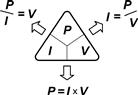
Figure 1.6 Triangle showing the relationship between P, I and V
The relationship, P = I × V, may be combined with that which results from Ohm’s Law (V = I × R) to produce two further relationships. First, substituting for V gives:
![]()
Secondly, substituting for I gives:
![]()
Example 1.19
A current of 1.5A is drawn from a 3V battery. What power is supplied?
Solution
Here we must use P = I × V (where I = 1.5A and V = 3V).
![]()
Hence, a power of 4.5W is supplied.
Example 1.20
A voltage drop of 4V appears across a resistor of 100Ω. What power is dissipated in the resistor?
Solution
Here we use P = V2/R (where V = 4V and R = 100Ω).
![]()
Hence, the resistor dissipates a power of 0.16W (or 160 mW).
Example 1.21
A current of 20 mA flows in a 1 kΩ resistor. What power is dissipated in the resistor?
Solution
Here we use P = I2 × R but, to make life a little easier, we will work in mA and kΩ (in which case the answer will be in mW).
![]()
Thus, a power of 400 mW is dissipated in the 1 kΩ resistor.
1.1.13 Electrostatics
If a conductor has a deficit of electrons, it will exhibit a net positive charge. If, on the other hand, it has a surplus of electrons, it will exhibit a net negative charge. An imbalance in charge can be produced by friction (removing or depositing electrons using materials such as silk and fur, respectively), or induction (by attracting or repelling electrons using a second body, which is, respectively, positively or negatively charged).
1.1.14 Force Between Charges
Coulomb’s Law states that, if charged bodies exist at two points, the force of attraction (if the charges are of opposite polarity), or repulsion (if the charges have the same polarity), will be proportional to the product of the magnitude of the charges divided by the square of their distance apart. Thus:
![]()
where Q1 and Q2 are the charges present at the two points (in coulombs), r the distance separating the two points (in meters), F is the force (in newtons), and k is a constant depending upon the medium in which the charges exist.
In vacuum or “free space”:

where ε0 is the permittivity of free space (8.854 × 10⁻¹² C/Nm2).
Combining the two previous equations gives:
![]()
1.1.15 Electric Fields
The force exerted on a charged particle is a manifestation of the existence of an electric field. The electric field defines the direction and magnitude of a force on a charged object. The field itself is invisible to the human eye, but can be drawn by constructing lines, which indicate the motion of a free positive charge within the field; the number of field lines in a particular region being used to indicate the relative strength of the field at the point in question.
Figures 1.7 and 1.8 show the electric fields between charges of the same and opposite polarity, while Figure 1.9 shows the field that exists between two charged parallel plates. You will see more of this particular arrangement when we introduce capacitors.

Figure 1.7 Electric field between two unlike electric charges

Figure 1.8 Electric field between two like electric charges (in this case both positive)

Figure 1.9 Electric field between two parallel plates
1.1.16 Electric Field Strength
The strength of an electric field (E) is proportional to the applied potential difference and inversely proportional to the distance between the two conductors. The electric field strength is given by:
![]()
where E is the electric field strength (V/m), V is the applied potential difference (V) and d is the distance (m).
Example 1.22
Two parallel conductors are separated by a distance of 25 mm. Determine the electric field strength if they are fed from a 600V DC supply.
Solution
The electric field strength will be given by:
![]()
1.1.17 Permittivity
The amount of charge produced on the two plates shown in Figure 1.9 for a given applied voltage will depend not only on the physical dimensions, but also on the insulating dielectric material that appears between the plates. Such materials need to have a very high value of resistivity (they must not conduct charge) coupled with an ability to withstand high voltages without breaking down.
A more practical arrangement is shown in Figure 1.10. In this arrangement the ratio of charge, Q, to potential difference, V, is given by the relationship:
![]()
where A is the surface area of the plates (in m), d is the separation (in m), and ε is a constant for the dielectric material known as the absolute permittivity of the material (sometimes also referred to as the dielectric constant).

Figure 1.10 Parallel plates with an insulating dielectric material
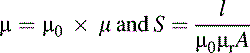
The absolute permittivity of a dielectric material is the product of the permittivity of free space (ε0) and the relative permittivity (εr) of the material. Thus:
![]()
The dielectric strength of an insulating dielectric is the maximum electric field strength that can safely be applied to it before breakdown (conduction) occurs. Table 1.6 shows values of relative permittivity and dielectric strength for some common dielectric materials.
Table 1.6 Properties of some common insulating dielectric materials
| Dielectric material | Relative permittivity (free space = 1) | Dielectric strength (kV/mm) |
| Vacuum, or free space | 1 | ∞ |
| Air | 1 | 3 |
| Polythene | 2.3 | 50 |
| Paper | 2.5 to 3.5 | 14 |
| Polystyrene | 2.5 | 25 |
| Mica | 4 to 7 | 160 |
| Pyrex glass | 4.5 | 13 |
| Glass ceramic | 5.9 | 40 |
| Polyester | 3.0 to 3.4 | 18 |
| Porcelain | 6.5 | 4 |
| Titanium dioxide | 100 | 6 |
| Ceramics | 5 to 1,000 | 2 to 10 |
1.1.18 Electromagnetism
When a current flows through a conductor, a magnetic field is produced in the vicinity of the conductor. The magnetic field is invisible, but its presence can be detected using a compass needle (which will deflect from its normal North-South position). If two current-carrying conductors are placed in the vicinity of one another, the fields will interact with one another and the conductors will experience a force of attraction or repulsion (depending upon the relative direction of the two currents).
1.1.19 Force Between Two Current-Carrying Conductors
The mutual force that exists between two parallel current-carrying conductors will be proportional to the product of the currents in the two conductors and the length of the conductors but inversely proportional to their separation. Thus:
![]()
where I1 and I2 are the currents in the two conductors (in amps), l is the parallel length of the conductors (in meters), d is the distance separating the two conductors (in meters), F is the force (in newtons), and k is a constant depending upon the medium in which the charges exist.
In vacuum or “free space”,
![]()
where μ0 is a constant known as the permeability of free space (4π × 10−7 or 12.57 × 10⁻⁷H/m).
Combining the two previous equations gives:
![]()
or,

or,

1.1.20 Magnetic Fields
The field surrounding a straight current-carrying conductor is shown in Figure 1.11. The magnetic field defines the direction of motion of a free North Pole within the field. In the case of Figure 1.11, the lines of flux are concentric and the direction of the field determined by the direction of current flow) is given by the right-hand rule.
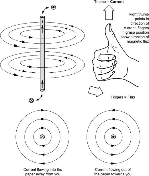
Figure 1.11 Magnetic field surrounding a straight conductor
1.1.21 Magnetic Field Strength
The strength of a magnetic field is a measure of the density of the flux at any particular point. In the case of Figure 1.11, the field strength will be proportional to the applied current and inversely proportional to the perpendicular distance from the conductor. Thus:
![]()
where B is the magnetic flux density (in tesla), I is the current (in amperes), d is the distance from the conductor (in meters), and k is a constant.
Assuming that the medium is vacuum or “free space,” the density of the magnetic flux will be given by:
![]()
where B is the flux density (in tesla), μ0 is the permeability of free space (4π × 10−7 or 12.57 × 10⁻⁷), I is the current (in amperes), and d is the distance from the center of the conductor (in meters).
The flux density is also equal to the total flux divided by the area of the field. Thus:
![]()
where Φ is the flux (in webers) and A is the area of the field (in square meters).
In order to increase the strength of the field, a conductor may be shaped into a loop (Figure 1.12) or coiled to form a solenoid (Figure 1.13). Note, in the latter case, how the field pattern is exactly the same as that which surrounds a bar magnet.

Figure 1.12 Forming a conductor into a loop increases the strength of the magnetic field in the center of the loop

Figure 1.13 The magnetic field surrounding a solenoid coil resembles that of a permanent magnet
Example 1.23
Determine the flux density produced at a distance of 50 mm from a straight wire carrying a current of 20A.
Solution
Applying the formula B = μ0I/2π d gives:

from which:
![]()
Thus, B = 80 × 10−6 T or B = 80 μT.
Example 1.24
A flux density of 2.5 mT is developed in free space over an area of 20 cm2. Determine the total flux.
Solution
Rearranging the formula B = Φ/A to make Φ the subject gives Φ = B × A thus:
![]()
from which B = 5 μWb
1.22 Magnetic Circuits
Materials such as iron and steel possess considerably enhanced magnetic properties. They are employed in applications where it is necessary to increase the flux density produced by an electric current. In effect, magnetic materials allow us to channel the electric flux into a “magnetic circuit,” as shown in Figure 1.14.

Figure 1.14 Comparison of electric and magnetic circuits
In the circuit of Figure 1.14(B), the reluctance of the magnetic core is analogous to the resistance present in the electric circuit shown in Figure 1.14(A). We can make the following comparisons between the two types of circuit (see Table 1.7).
Table 1.7 Comparison of electric and magnetic circuits
| Electric circuit Figure 1.14(A) | Magnetic circuit Figure 1.14(A) |
| Electromotive force, e.m.f. = V | Magnetomotive force, m.m.f. = N × I |
| Resistance = R | Reluctance = S |
| Current = I | Flux = Φ |
| e.m.f. = current × resistance | m.m.f. = flux × reluctance |
| V = I × R | N I = S Φ |
In practice, not all of the magnetic flux produced in a magnetic circuit will be concentrated within the core and some “leakage flux” will appear in the surrounding free space (as shown in Figure 1.15). Similarly, if a gap appears within the magnetic circuit, the flux will tend to spread out as shown in Figure 1.16. This effect is known as fringing.
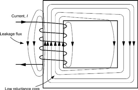
Figure 1.15 Leakage flux in a magnetic circuit

Figure 1.16 Fringing of the magnetic flux at an air gap in a magnetic circuit
1.1.23 Reluctance and Permeability
The reluctance of a magnetic path is directly proportional to its length and inversely proportional to its area. The reluctance is also inversely proportional to the absolute permeability of the magnetic material. Thus:

where S is the reluctance of the magnetic path, l is the length of the path (in meters), A is the cross-sectional area of the path (in square meters), and μ is the absolute permeability of the magnetic material.
The absolute permeability of a magnetic material is the product of the permeability of free space (μ0) and the relative permeability of the magnetic medium (μ0). Thus:
The permeability of a magnetic medium is a measure of its ability to support magnetic flux and it is equal to the ratio of flux density (B) to magnetizing force (H). Thus:
![]()
where B is the flux density (in tesla) and H is the magnetizing force (in ampere/meter). The magnetizing force (H) is proportional to the product of the number of turns and current but inversely proportional to the length of the magnetic path.
![]()
where H is the magnetizing force (in amperes/meters), N is the number of turns, I is the current (in amperes), and l is the length of the magnetic path (in meters).
1.1.24 B-H Curves
Figure 1.17 shows four typical B-H (flux density plotted against permeability) curves for some common magnetic materials. If you look carefully at these curves you will notice that they flatten off due to magnetic saturation and that the slope of the curve (indicating the value of μ corresponding to a particular value of H) falls as the magnetizing force increases. This is important since it dictates the acceptable working range for a particular magnetic material when used in a magnetic circuit.

Figure 1.17 B-H curves for three ferromagnetic materials
Example 1.25
Estimate the relative permeability of cast steel (see Figure 1.18) at (a) a flux density of 0.6T, and (b) a flux density of 1.6T.

Figure 1.18 B-H curve for a sample of cast steel
Solution
From Figure 1.18, the slope of the graph at any point gives the value of μ at that point. We can easily find the slope by constructing a tangent at the point in question and then finding the ratio of vertical change to horizontal change.
(a) The slope of the graph at 0.6T is 0.6/800 = 0.75 × 10⁻³
Since μ = μ0 × μr, μr = μ/μ0 = 0.75 × 10⁻³/12.57 × 10−7, thus μr = 597 at 0.6T.
(b) The slope of the graph at 1.6T is 0.2/4,000 = 0.05 × 10⁻³
Since μ = μ0 × μr, μr = μ/μ0 = 0.05 × 10⁻³ / 12.57 × 10⁻⁷, thus μr = 39.8 at 1.6T.
(This example clearly shows the effect of saturation on the permeability of a magnetic material!)
Example 1.26
A coil of 800 turns is wound on a closed mild steel core having a length 600 mm and cross-sectional area 500 mm2. Determine the current required to establish a flux of 0.8 mWb in the core.
Solution
Now B = Φ/A = (0.8 × 10⁻³)/(500 × 10−6) = 1.6T
From Figure 1.17, a flux density of 1.6T will occur in mild steel when H = 3,500 A/m. The current can now be determined by re-arranging H = N I/l as follows:
![]()
1.1.25 Circuit Diagrams
Finally, and just in case you haven’t seen them before, we will end this section with a brief word about circuit diagrams. We are introducing the topic here because it’s quite important to be able to read and understand simple electronic circuit diagrams before you can make sense of some of the components and circuits that you will meet later on.
Circuit diagrams use standard symbols and conventions to represent the components and wiring used in an electronic circuit. Visually, they bear very little relationship to the physical layout of a circuit but, instead, they provide us with a “theoretical” view of the circuit. In this section we show you how to find your way around simple circuit diagrams.
To be able to understand a circuit diagram you first need to be familiar with the symbols that are used to represent the components and devices. It’s important to be aware that there are a few (thankfully quite small) differences between the symbols used in circuit diagrams of American and European origin.
As a general rule, the input to a circuit should be shown on the left of a circuit diagram and the output shown on the right. The supply (usually the most positive voltage) is normally shown at the top of the diagram and the common, 0V, or ground connection is normally shown at the bottom. This rule is not always obeyed, particularly for complex diagrams where many signals and supply voltages may be present.
Note also that, in order to simplify a circuit diagram (and avoid having too many lines connected to the same point) multiple connections to common, 0V, or ground may be shown using the appropriate symbol. The same applies to supply connections that may be repeated (appropriately labeled) at various points in the diagram.
A very simple circuit diagram (a simple resistance tester) is shown in Figure 1.20. This circuit may be a little daunting if you haven’t met a circuit like it before but you can still glean a great deal of information from the diagram even if you don’t know what the individual components do.

Figure 1.19 Various types of switches. From left to right: a mains rocker switch, an SPDT miniature toggle (changeover) switch, a DPDT side switch, an SPDT push-button (wired for use as an SPST push-button), a miniature PCB mounting DPDT push-button (with a latching action).

Figure 1.20 A simple circuit diagram
The circuit uses two batteries, B1 (a 9V multi-cell battery) and B2 (a 1.5V single-cell battery). The two batteries are selected by means of a double-pole, double-throw (DPDT) switch. This allows the circuit to operate from either the 9V battery (B1) as shown in Figure 1.20(A) or from the 1.5V battery (B2) as shown in Figure 1.20(B) depending on the setting of S1.
A variable resistor, VR1, is used to adjust the current supplied by whichever of the two batteries is currently selected. This current flows first through VR1, then through the milliammeter, and finally through the unknown resistor, RX. Notice how the meter terminals are labeled showing their polarity (the current flows into the positive terminal and out of the negative terminal).
The circuit shown in Figure 1.20(C) uses a different type of switch but provides exactly the same function. In this circuit a single-pole, double-throw (SPDT) switch is used and the negative connections to the two batteries are “commoned” (i.e., connected directly together).
Finally, Figure 1.20(D) shows how the circuit can be redrawn using a common “chassis” connection to provide the negative connection between RX and the two batteries. Electrically this circuit is identical to the one shown in Figure 1.20(C).
1.2 Passive Components
This section introduces several of the most common types of electronic component, including resistors, capacitors and inductors. These are often referred to as passive components as they cannot, by themselves, generate voltage or current. An understanding of the characteristics and application of passive components is an essential prerequisite to understanding the operation of the circuits used in amplifiers, oscillators, filters and power supplies.
1.2.1 Resistors
The notion of resistance as opposition to current was discussed in the previous section. Conventional forms of resistor obey a straight line law when voltage is plotted against current (see Figure 1.21) and this allows us to use resistors as a means of converting current into a corresponding voltage drop, and vice versa (note that doubling the applied current will produce double the voltage drop, and so on). Therefore, resistors provide us with a means of controlling the currents and voltages present in electronic circuits. They can also act as loads to simulate the presence of a circuit during testing (e.g., a suitably rated resistor can be used to replace a loudspeaker when an audio amplifier is being tested).

Figure 1.21 Voltage plotted against current for three different values of resistor
The specifications for a resistor usually include the value of resistance expressed in ohms (Ω), kilohms (kΩ) or megohms (MΩ), the accuracy or tolerance (quoted as the maximum permissible percentage deviation from the marked value), and the power rating (which must be equal to, or greater than, the maximum expected power dissipation).
Other practical considerations when selecting resistors for use in a particular application include temperature coefficient, noise performance, stability and ambient temperature range. Table 1.8 summarizes the properties of five of the most common types of resistor. Figure 1.22 shows a typical selection of fixed resistors with values from 15Ω to 4.7 kΩ.
Table 1.8 Characteristics of common types of resistors


Figure 1.22 A selection of resistors including high-power metal clad, ceramic wirewound, carbon and metal film types with values ranging from 15Ω to 4.7 kΩ
1.2.2 Preferred Values
The value marked on the body of a resistor is not its exact resistance. Some minor variation in resistance value is inevitable due to production tolerance. For example, a resistor marked 100Ω and produced within a tolerance of ±10% will have a value which falls within the range 90Ω to 110Ω. A similar component with a tolerance of ±1% would have a value that falls within the range 99Ω to 101Ω. Thus, where accuracy is important it is essential to use close tolerance components.
Resistors are available in several series of fixed-decade values, the number of values provided with each series being governed by the tolerance involved. In order to cover the full range of resistance values using resistors having a ±20% tolerance it will be necessary to provide six basic values (known as the E6 series). More values will be required in the series, which offers a tolerance of ±10%, and consequently, the E12 series provides twelve basic values. The E24 series for resistors of ±5% tolerance provides no fewer than 24 basic values and, as with the E6 and E12 series, decade multiples (i.e., ×1, ×10, ×100, ×1 k, ×10 k, ×100k and ×1M) of the basic series. Figure 1.23 shows the relationship between the E6, E12 and E24 series.

Figure 1.23 The E6, E12, and E24 series
1.2.3 Power Ratings
Resistor power ratings are related to operating temperatures and resistors should be derated at high temperatures. Where reliability is important resistors should be operated at well below their nominal maximum power dissipation.
Example 1.27
A resistor has a marked value of 220Ω. Determine the tolerance of the resistor if it has a measured value of 207Ω.
Solution
The difference between the marked and measured values of resistance (the error) is (220Ω − 207Ω) = 13Ω. The tolerance is given by:
![]()
The tolerance is thus, (13/220) × 100 = 5.9%.
Example 1.28
A 9V power supply is to be tested with a 39Ω load resistor. If the resistor has a tolerance of 10% find:
Solution
(a) If a resistor of exactly 39Ω is used the current will be:
![]()
(b) The lowest value of resistance would be (39Ω − 3.9Ω) = 35.1Ω. In which case the current would be:
![]()
At the other extreme, the highest value would be (39Ω + 3.9 Ω) = 42.9Ω.
In this case, the current would be:
![]()
The maximum and minimum values of supply current will thus be 256.4 mA and 209.8 mA, respectively.
Example 1.29
A current of 100 mA (±20%) is to be drawn from a 28V DC supply. What value and type of resistor should be used in this application?
Solution
The value of resistance required must first be calculated using Ohm’s Law:
![]()
The nearest preferred value from the E12 series is 270Ω (which will actually produce a current of 103.7 mA (i.e., within ±4% > of the desired value). If a resistor of ±10% tolerance is used, current will be within the range 94 mA to 115 mA (well within the ±20% accuracy specified).
The power dissipated in the resistor (calculated using P = I × V) will be 2.9W and thus a component rated at 3W (or more) will be required. This would normally be a vitreous enamel coated wirewound resistor (see Table 1.8).
1.2.4 Resistor Markings
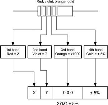
Carbon and metal oxide resistors are normally marked with color codes which indicate their value and tolerance. Two methods of color-coding are in common use; one involves four colored bands (see Figure 1.24), while the other uses five color bands (see Figure 1.25).

Figure 1.24 Four-band resistor color code

Figure 1.25 Five band resistor color code
Example 1.30
A resistor is marked with the following colored stripes: brown, black, red, silver. What is its value and tolerance?

Example 1.31
A resistor is marked with the following colored stripes: red, violet, orange, gold. What is its value and tolerance?
Example 1.32
A resistor is marked with the following colored stripes: green, blue, black, gold. What is its value and tolerance?

Example 1.33
A resistor is marked with the following colored stripes: red, green, black, black, brown. What is its value and tolerance?

Example 1.34
A 2.2 kΩ of ±2% tolerance is required. What four-band color code does this correspond to?
Solution
Red (2), red (2), red (2 zeros), red (2% tolerance). Thus, all four bands should be red.
1.2.5 BS 1852 Coding
Some types of resistor have markings based on a system of coding defined in BS 1852. This system involves marking the position of the decimal point with a letter to indicate the multiplier concerned as shown in Table 1.9. A further letter is then appended to indicate the tolerance as shown in Table 1.10.
Table 1.9 BS 1852 resistor multiplier markings
| Letter | Multiplier |
| R | 1 |
| K | 1,000 |
| M | 1,000,000 |
Table 1.10 BS 1852 resistor tolerance markings
| Letter | Multiplier |
| F | ±1% |
| G | ±2% |
| J | ±5% |
| K | ±10% |
| M | ±20% |
Solution
4.7Ω ± 10%
Example 1.36
A resistor is marked coded with the legend 330RG. What is its value and tolerance?
Solution
330Ω ± 2%
Example 1.37
A resistor is marked coded with the legend R22M. What is its value and tolerance?
Solution
0.22Ω ± 20%
1.2.6 Series and Parallel Combinations of Resistors
In order to obtain a particular value of resistance, fixed resistors may be arranged in either series or parallel as shown in Figures 1.30 and 1.31.
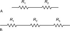
Figure 1.30 Resistors in series

Figure 1.31 Resistors in parallel
The effective resistance of each of the series circuits shown in Figure 1.30 is simply equal to the sum of the individual resistances. So, for the circuit shown in Figure 1.30(A):
![]()
while for Figure 1.30(B):
![]()
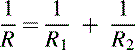
Turning to the parallel resistors shown in Figure 1.31, the reciprocal of the effective resistance of each circuit is equal to the sum of the reciprocals of the individual resistances. Hence, for Figure 1.31(A):
while for Figure 1.32(B):


Figure 1.32 See Example 1.39
In the former case, the formula can be more conveniently rearranged as follows:

You can remember this as the product of the two resistance values divided by the sum of the two resistance values.
Example 1.38
Resistors of 22Ω, 47Ω, and 33Ω are connected (a) in series and (b) in parallel. Determine the effective resistance in each case.

Example 1.39
Determine the effective resistance of the circuit shown in Figure 1.32.
Solution
The circuit can be progressively simplified as shown in Figure 1.33. The stages in this simplification are:
(a) R3 and R4 are in series and they can replaced by a single resistance (RA) of (12Ω + 27Ω) = 39Ω.
(b) RA appears in parallel with R2. These two resistors can be replaced by a single resistance (RB) of (39Ω + 47Ω)/(39Ω + 47Ω) = 21.3Ω.
(c) RB appears in series with R1. These two resistors can be replaced by a single resistance (R) of (21.3Ω + 4.7Ω) = 26Ω.

Figure 1.33 See Example 1.39
Example 1.40
A resistance of 50Ω rated at 2W is required. What parallel combination of preferred value resistors will satisfy this requirement? What power rating should each resistor have?
Solution
Two 100Ω resistors may be wired in parallel to provide a resistance of 50Ω as shown below:

Note, from this, that when two resistors of the same value are connected in parallel the resulting resistance will be half that of a single resistor.
Having shown that two 100Ω resistors connected in parallel will provide us with a resistance of 50Ω we now need to consider the power rating. Since the resistors are identical, the applied power will be shared equally between them. Hence, each resistor should have a power rating of 1W.
1.2.7 Resistance and Temperature
Figure 1.34 shows how the resistance of a metal conductor (e.g., copper) varies with temperature. Since the resistance of the material increases with temperature, this characteristic is said to exhibit a positive temperature coefficient (PTC). Not all materials have a PTC characteristic. The resistance of a carbon conductor falls with temperature and it is therefore said to exhibit a negative temperature coefficient (NTC).

Figure 1.34 Variation of resistance with temperature for a metal conductor
The resistance of a conductor at a temperature, t, is given by the equation:
![]()
where α, β, γ, etc. are constants and R0 is the resistance at 0°C.
The coefficients, β, γ, etc. are quite small and since we are normally only dealing with a relatively restricted temperature range (e.g., 0 °C to 100 °C), we can usually approximate the characteristic shown in Figure 1.34 to the straight line law shown in Figure 1.35. In this case, the equation simplifies to:
![]()
where α is known as the temperature coefficient of resistance. Table 1.11 shows some typical values for α (note that α is expressed in Ω/Ω/°C or just /°C).

Figure 1.35 Straight line approximation of Figure 1.34
Table 1.11 Temperature coefficient of resistance
| Material | Temperature coefficient of resistance, α (/°C) |
| Platinum | +0.0034 |
| Silver | +0.0038 |
| Copper | +0.0043 |
| Iron | +0.0065 |
| Carbon | −0.0005 |
Example 1.41
A resistor has a temperature coefficient of 0.001/°C. If the resistor has a resistance of 1.5 kΩ at 0 °C, determine its resistance at 80 °C.
Example 1.42
A resistor has a temperature coefficient of 0.0005/°C. If the resistor has a resistance of 680Ω at 20 °C, what will its resistance be at 80 °C?
Solution
First we must find the resistance at 0°C. Rearranging the formula for Rt gives:
Hence,
![]()
Now,
![]()
thus,
![]()
Hence,
![]()
Example 1.43
A resistor has a resistance of 40Ω at 0°C and 44Ω at 100°C. Determine the resistor’s temperature coefficient.
Solution
First we need to make α the subject of the formula:
![]()
Now,

from which,
![]()
1.2.8 Thermistors
With conventional resistors we would normally require resistance to remain the same over a wide range of temperatures (i.e., α should be zero). On the other hand, there are applications in which we could use the effect of varying resistance to detect a temperature change. Components that allow us to do this are known as thermistors. The resistance of a thermistor changes markedly with temperature and these components are widely used in temperature sensing and temperature compensating applications. Two basic types of thermistor are available, NTC and PTC (see Figure 1.36).

Figure 1.36 Characteristics of (A) NTC and (B) PTC thermistors
Typical NTC thermistors have resistances that vary from a few hundred (or thousand) ohms at 25 °C to a few tens (or hundreds) of ohms at 100 °C. PTC thermistors, on the other hand, usually have a resistance-temperature characteristic that remains substantially flat (typically at around 100Ω) over the range 0 °C to around 75 °C. Above this, and at a critical temperature (usually in the range 80 °C to 120 °C) their resistance rises very rapidly to values of up to, and beyond, 10 kΩ (see Figure 1.36).
A typical application of PTC thermistors is over-current protection. Provided the current passing through the thermistor remains below the threshold current, the effects of self-heating will remain negligible and the resistance of the thermistor will remain low (i.e., approximately the same as the resistance quoted at 25 °C). Under fault conditions, the current exceeds the threshold value by a considerable margin and the thermistor starts to self-heat. The resistance then increases rapidly and, as a consequence, the current falls to the rest value. Typical values of threshold and rest currents are 200 mA and 8 mA, respectively, for a device which exhibits a nominal resistance of 25Ω at 25 °C.
1.2.9 Light-Dependent Resistors
Light-dependent resistors (LDR) use a semiconductor material (i.e., a material that is neither a conductor nor an insulator) whose electrical characteristics vary according to the amount of incident light. The two semiconductor materials used for the manufacture of LDRs are cadmium sulphide (CdS) and cadmium selenide (CdSe). These materials are most sensitive to light in the visible spectrum, peaking at about 0.6 μm for CdS and 0.75 μm for CdSe. A typical CdS LDR exhibits a resistance of around 1 MΩ in complete darkness and less than 1 kΩ when placed under a bright light source (see Figure 1.37).

Figure 1.37 Characteristic of a light-dependent resistor (LDR)
1.2.10 Voltage Dependent Resistors
The resistance of a voltage dependent resistor (VDR) falls very rapidly when the voltage across it exceeds a nominal value in either direction (see Figure 1.38). In normal operation, the current flowing in a VDR is negligible; however, when the resistance falls, the current will become appreciable and a significant amount of energy will be absorbed. VDRs are used as a means of “clamping” the voltage in a circuit to a predetermined level. When connected across the supply rails to a circuit (either AC or DC) they are able to offer a measure of protection against voltage surges.
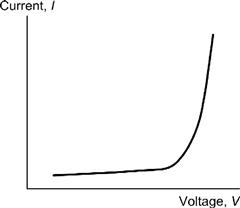
Figure 1.38 Characteristic of a voltage dependent resistor (VDR)
1.2.11 Variable Resistors
Variable resistors are available in several forms including those which use carbon tracks and those which use a wirewound resistance element. In either case, a moving slider makes contact with the resistance element. Most variable resistors have three (rather than two) terminals and as such are more correctly known as potentiometers. Carbon potentiometers are available with linear or semi-logarithmic law tracks (see Figure 1.39) and in rotary or slider formats. Ganged controls, in which several potentiometers are linked together by a common control shaft, are also available. Figure 1.40 shows a selection of variable resistors.

Figure 1.39 Characteristics for linear and semi-logarithmic law variable resistors

Figure 1.40 A selection of common types of carbon and wirewound variable resistors/potentiometers
You will also encounter various forms of preset resistors that are used to make occasional adjustments (e.g., for calibration). Various forms of preset resistor are commonly used including open carbon track skeleton presets and fully encapsulated carbon and multiturn cermet types, as shown in Figure 1.41.
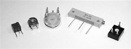
Figure 1.41 A selection of common types of standard and miniature preset resistors/potentiometers
1.2.12 Capacitors
A capacitor is a device for storing electric charge. In effect, it is a reservoir into which charge can be deposited and then later extracted. Typical applications include reservoir and smoothing capacitors for use in power supplies, coupling AC signals between the stages of amplifiers, and decoupling supply rails (i.e., effectively grounding the supply rails as far as AC signals are concerned).
A capacitor can consist of nothing more than two parallel metal plates as shown in Figure 1.10. To understand what happens when a capacitor is being charged and discharged take a look at Figure 1.42. If the switch is left open (position A), no charge will appear on the plates and in this condition there will be no electric field in the space between the plates nor will there be any charge stored in the capacitor.

Figure 1.42 Capacitor charging and discharging
When the switch is moved to position B, electrons will be attracted from the positive plate to the positive terminal of the battery. At the same time, a similar number of electrons will move from the negative terminal of the battery to the negative plate. This sudden movement of electrons will manifest itself in a momentary surge of current (conventional current will flow from the positive terminal of the battery toward the positive terminal of the capacitor).
Eventually, enough electrons will have moved to make the e.m.f. between the plates the same as that of the battery. In this state, the capacitor is said to be fully charged and an electric field will be present in the space between the two plates.
If at some later time the switch is moved back to position A, the positive plate will be left with a deficiency of electrons while the negative plate will be left with a surplus of electrons. Furthermore, since there is no path for current to flow between the two plates the capacitor will remain charged and a potential difference will be maintained between the plates.
Now assume that the switch is moved to position C. The excess electrons on the negative plate will flow through the resistor to the positive plate until a neutral state once again exists (i.e., until there is no excess charge on either plate). In this state the capacitor is said to be fully discharged and the electric field between the plates will rapidly collapse. The movement of electrons during the discharging of the capacitor will again result in a momentary surge of current (current will flow from the positive terminal of the capacitor and into the resistor).
Figure 1.43 shows the direction of current flow in the circuit of Figure 1.42 during charging (switch in position B) and discharging (switch in position C). It should be noted that current flows momentarily in both circuits even though you may think that the circuit is broken by the gap between the capacitor plates!
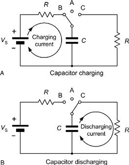
Figure 1.43 Current flow during charging and discharging
1.2.13 Capacitance
The unit of capacitance is the farad (F). A capacitor is said to have a capacitance of 1F if a current of 1A flows in it when a voltage changing at the rate of 1 V/s is applied to it. The current flowing in a capacitor will thus be proportional to the product of the capacitance, C, and the rate of change of applied voltage. Hence:
![]()
Note that we’ve used a small i to represent the current flowing in the capacitor. We’ve done this because the current is changing and doesn’t remain constant.
The rate of change of voltage is often represented by the expression dv/dt where dv represents a very small change in voltage and dt represents the corresponding small change in time. Expressing this mathematically gives:
![]()
Example 1.44
A voltage is changing at a uniform rate from 10V to 50V in a period of 0.1s. If this voltage is applied to a capacitor of 22 μF, determine the current that will flow.
Solution
Now the current flowing will be given by:
![]()
Thus,

From which,
so,
![]()
1.2.14 Charge, Capacitance and Voltage
The charge or quantity of electricity that can be stored in the electric field between the capacitor plates is proportional to the applied voltage and the capacitance of the capacitor. Thus:
![]()
where Q is the charge (in coulombs), C is the capacitance (in farads), and V is the potential difference (in volts).
1.2.15 Energy storage
The energy stored in a capacitor is proportional to the product of the capacitance and the square of the potential difference. Thus:
![]()
where W is the energy (in joules), C is the capacitance (in farads), and V is the potential difference (in volts).
Example 1.46
A capacitor of 47 μF is required to store 4J of energy. Determine the potential difference that must be applied to the capacitor.
Solution
The foregoing formula can be rearranged to make V the subject as follows:

from which,

1.2.16 Capacitance and Physical Dimensions
The capacitance of a capacitor depends upon the physical dimensions of the capacitor (i.e., the size of the plates and the separation between them) and the dielectric material between the plates. The capacitance of a conventional parallel plate capacitor is given by:
![]()
where C is the capacitance (in farads), ε0 is the permittivity of free space, εr is the relative permittivity of the dielectric medium between the plates), and d is the separation between the plates (in meters).
Example 1.47
A capacitor of 1 nF is required. If a dielectric material of thickness 0.1 mm and relative permittivity 5.4 is available, determine the required plate area.
Solution
Rearranging the formula:
![]()
to make A the subject gives:

from which:

thus,
![]()
In order to increase the capacitance of a capacitor, many practical components employ multiple plates (see Figure 1.44). The capacitance is then given by:
![]()
where C is the capacitance (in farads), ε0 is the permittivity of free space, εr is the relative permittivity of the dielectric medium between the plates), and d is the separation between the plates (in meters) and n is the total number of plates.

Figure 1.44 A multi-plate capacitor
Example 1.48
A capacitor consists of six plates each of area 20 cm2 separated by a dielectric of relative permittivity 4.5 and thickness 0.2 mm. Determine the value of capacitance.
Solution
Using:
![]()
gives:

from which,

Thus,
![]()
1.2.17 Capacitor Specifications
The specifications for a capacitor usually include the value of capacitance (expressed in microfarads, nanofarads or picofarads), the voltage rating (i.e., the maximum voltage which can be continuously applied to the capacitor under a given set of conditions), and the accuracy or tolerance (quoted as the maximum permissible percentage deviation from the marked value).
Other practical considerations when selecting capacitors for use in a particular application include temperature coefficient, leakage current, stability and ambient temperature range.
Table 1.12 summarizes the properties of five of the most common types of capacitor. Note that electrolytic capacitors require the application of a polarizing voltage in order to the chemical action on which they depend for their operation.
Table 1.12 Characteristics of common types of capacitor

The polarizing voltages used for electrolytic capacitors can range from as little as 1V to several hundred volts depending upon the working voltage rating for the component in question.
Figure 1.45 shows some typical nonelectrolytic capacitors (including polyester, polystyrene, ceramic and mica types), while Figure 1.46 shows a selection of electrolytic (polarized) capacitors. An air-spaced variable capacitor is shown later in Figure 1.54.

Figure 1.45 A typical selection of nonelectrolytic capacitors (including polyester, polystyrene, ceramic and mica types) with values ranging from 10 pF to 470 nF and working voltages from 50V to 250V
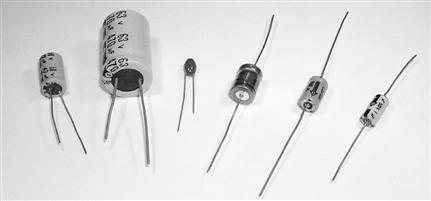
Figure 1.46 A typical selection of electrolytic (polarized) capacitors with values ranging from 1 μF to 470 μF and working voltages from 10V to 63V
1.2.18 Capacitor Markings
The vast majority of capacitors employ written markings which indicate their values, working voltages, and tolerance. The most usual method of marking resin dipped polyester (and other) types of capacitor involves quoting the value (μF, nF or pF), the tolerance (often either 10% or 20%), and the working voltage (often using _ and ∼ to indicate DC and AC, respectively). Several manufacturers use two separate lines for their capacitor markings and these have the following meanings:
First line:capacitance (pF or μF) and tolerance (K = 10%, M = 20%)
Second line: rated DC voltage and code for the dielectric material
A three-digit code is commonly used to mark monolithic ceramic capacitors. The first two digits of this code correspond to the first two digits of the value, while the third digit is a multiplier which gives the number of zeros to be added to give the value in picofarads. Other capacitors may use a color code similar to that used for marking resistor values (see Figure 1.48).
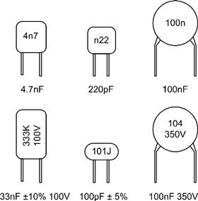
Figure 1.47 Examples of capacitor markings

Figure 1.48 Capacitor color code
Solution
The value (pF) will be given by the first two digits (10) followed by the number of zeros indicated by the third digit (3). The value of the capacitor is thus 10,000 pF or 10 nF. The final letter (K) indicates that the capacitor has a tolerance of 10%.

1.2.19 Series and Parallel Combination of Capacitors
In order to obtain a particular value of capacitance, fixed capacitors may be arranged in either series or parallel (Figures 1.50 and 1.51). The reciprocal of the effective capacitance of each of the series circuits shown in Figure 1.50 is equal to the sum of the reciprocals of the individual capacitances. Hence, for Figure 1.50(A):
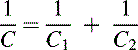
while for Figure 1.50(B):

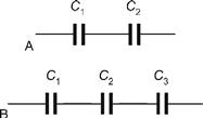
Figure 1.50 Capacitors in series

Figure 1.51 Capacitors in parallel
In the former case, the formula can be more conveniently rearranged as follows:

You can remember this as the product of the two capacitor values divided by the sum of the two values—just as you did for two resistors in parallel.
For a parallel arrangement of capacitors, the effective capacitance of the circuit is simply equal to the sum of the individual capacitances. Hence, for Figure 1.51(A):
![]()
while for Figure 1.51(B):
![]()
Example 1.51
Determine the effective capacitance of the circuit shown in Figure 1.52.

Figure 1.52 See Example 1.51
Solution
The circuit of Figure 1.52 can be progressively simplified as shown in Figure 1.53. The stages in this simplification are:
(a) C1 and C2 are in parallel and they can be replaced by a single capacitor (CA) of (2 nF + 4 nF) = 6 nF.
(b) CA appears in series with C3. These two resistors can be replaced by a single capacitor (CB) of (6 nF × 2 nF)/(6 nF + 2 nF) = 1.5 nF.
(c) CB appears in parallel with C4. These two capacitors can be replaced by a single capacitance (C) of (1.5 nF + 4 nF) = 5.5 nF.

Figure 1.53 See Example 1.51
Example 1.52
A capacitance of 50 μF (rated at 100V) is required. What series combination of preferred value capacitors will satisfy this requirement? What voltage rating should each capacitor have?
Solution
Two 100 μF capacitors wired in series will provide a capacitance of 50 μF, as follows:

Since the capacitors are of equal value, the applied DC potential will be shared equally between them. Thus each capacitor should be rated at 50V. Note that, in a practical circuit, we could take steps to ensure that the DC voltage was shared equally between the two capacitors by wiring equal, high-value (e.g., 100 kΩ) resistors across each capacitor.
1.2.20 Variable Capacitors
By moving one set of plates relative to the other, a capacitor can be made variable. The dielectric material used in a variable capacitor can be either air (see Figure 1.54) or plastic (the latter tend to be more compact). Typical values for variable capacitors tend to range from about 25 pF to 500 pF. These components are commonly used for tuning radio receivers.

Figure 1.54 An air-spaced variable capacitor. This component (used for tuning an AM radio) has two separate variable capacitors (each of 500 pF maximum) operated from a common control shaft.
1.2.21 Inductors
Inductors provide us with a means of storing electrical energy in the form of a magnetic field. Typical applications include chokes, filters and (in conjunction with one or more capacitors) frequency selective circuits. The electrical characteristics of an inductor are determined by a number of factors including the material of the core (if any), the number of turns, and the physical dimensions of the coil. Figure 1.55 shows the construction of a typical toroidal inductor wound on a ferrite (high permeability) core.

Figure 1.55 A practical coil contains inductance and resistance
In practice every coil comprises both inductance (L) and a small resistance (R). The circuit of Figure 1.56 shows these as two discrete components. In reality the inductance and the resistance (we often refer to this as a loss resistance because it’s something that we don’t actually want) are both distributed throughout the component but it is convenient to treat the inductance and resistance as separate components in the analysis of the circuit.
![]()
Figure 1.56 A practical coil contains inductance and a small amount of series loss resistance
To understand what happens when a changing current flows through an inductor, take a look at the circuit shown in Figure 1.57(A). If the switch is left open, no current will flow and no magnetic flux will be produced by the inductor. If the switch is closed, as shown in Figure 1.57(B), current will begin to flow as energy is taken from the supply in order to establish the magnetic field. However, the change in magnetic flux resulting from the appearance of current creates a voltage (an induced e.m.f.) across the coil which opposes the applied e.m.f. from the battery.

Figure 1.57 Flux and e.m.f. generated when a changing current is applied to an inductor
The induced e.m.f. results from the changing flux and it effectively prevents an instantaneous rise in current in the circuit. Instead, the current increases slowly to a maximum at a rate which depends upon the ratio of inductance (L) to resistance (R) present in the circuit.
After a while, a steady-state condition will be reached in which the voltage across the inductor will have decayed to zero and the current will have reached a maximum value determined by the ratio of V to R (i.e., Ohm’s Law). This is shown in Figure 1.57(C).
If, after this steady-state condition has been achieved, the switch is opened, as shown in Figure 1.57(D), the magnetic field will suddenly collapse and the energy will be returned to the circuit in the form of an induced back e.m.f., which will appear across the coil as the field collapses. For large values of magnetic flux and inductance this back e.m.f. can be extremely large!
1.2.22 Inductance
Inductance is the property of a coil which gives rise to the opposition to a change in the value of current flowing in it. Any change in the current applied to a coil/inductor will result in an induced voltage appearing across it. The unit of inductance is the henry (H) and a coil is said to have an inductance of 1H if a voltage of 1V is induced across it when a current changing at the rate of 1 A/s is flowing in it.
The voltage induced across the terminals of an inductor will thus be proportional to the product of the inductance (L) and the rate of change of applied current. Hence:
![]()
Note that the minus sign indicates the polarity of the voltage, i.e., opposition to the change.
The rate of change of current is often represented by the expression di/dt where di represents a very small change in current and dt represents the corresponding small change in time. Using mathematical notation to write this we arrive at:
![]()
You might like to compare this with the similar relationship that we obtained for the current flowing in a capacitor shown in Section 1.2.13.


1.2.23 Energy Storage
The energy stored in an inductor is proportional to the product of the inductance and the square of the current flowing in it. Thus:
![]()
where W is the energy (in joules), L is the capacitance (in henries), and I is the current flowing in the inductor (in amps).

1.2.24 Inductance and Physical Dimensions
The inductance of an inductor depends upon the physical dimensions of the inductor (e.g., the length and diameter of the winding), the number of turns, and the permeability of the material of the core. The inductance of an inductor is given by:

where L is the inductance (in henries), μ0 is the permeability of free space, μr is the relative permeability of the magnetic core, l is the mean length of the core (in meters), and A is the cross-sectional area of the core (in square meters).
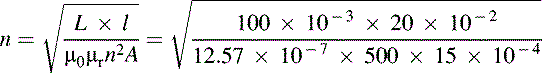
Example 1.55
An inductor of 100 mH is required. If a closed magnetic core of length 20 cm, cross-sectional area 15 cm2 and relative permeability 500 is available, determine the number of turns required.


1.2.25 Inductor Specifications
Inductor specifications normally include the value of inductance (expressed in henries, millihenries or microhenries), the current rating (i.e., the maximum current which can be continuously applied to the inductor under a given set of conditions), and the accuracy or tolerance (quoted as the maximum permissible percentage deviation from the marked value). Other considerations may include the temperature coefficient of the inductance (usually expressed in parts per million, p.p.m., per unit temperature change), the stability of the inductor, the DC resistance of the coil windings (ideally zero), the Q-factor (quality factor) of the coil, and the recommended working frequency range. Table 1.13 summarizes the properties of four common types of inductor. Some typical small inductors are shown in Figure 1.58. These have values of inductance ranging from 15 μH to 1 mH.
Table 1.13 Characteristics of common types of inductor


Figure 1.58 A selection of small inductors with values ranging from 15 μH to 1 mH
1.2.26 Inductor Markings
As with capacitors, the vast majority of inductors use written markings to indicate values, working current, and tolerance. Some small inductors are marked with colored stripes to indicate their value and tolerance (in which case the standard color values are used and inductance is normally expressed in microhenries).
1.2.27 Series and Parallel Combinations of Inductors
In order to obtain a particular value of inductance, fixed inductors may be arranged in either series or parallel as shown in Figs 1.59 and 1.60.
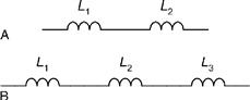
Figure 1.59 Inductors in series

Figure 1.60 Inductors in parallel
The effective inductance of each of the series circuits shown in Figure 1.59 is simply equal to the sum of the individual inductances. So, for the circuit shown in Figure 1.59(A):
![]()
while for Figure 1.59(B):
![]()
Turning to the parallel inductors shown in Figure 1.60, the reciprocal of the effective inductance of each circuit is equal to the sum of the reciprocals of the individual inductances. Hence, for Figure 1.60(A):
while for Figure 1.60(B):

In the former case, the formula can be more conveniently re-arranged as follows:

You can remember this as the product of the two inductance values divided by the sum of the two inductance values.
Example 1.56
An inductance of 5 mH (rated at 2A) is required. What parallel combination of preferred value inductors will satisfy this requirement?
Solution
Two 10 mH inductors may be wired in parallel to provide an inductance of 5 mH as shown below:

Since the inductors are identical, the applied current will be shared equally between them. Hence, each inductor should have a current rating of 1A.
Example 1.57
Determine the effective inductance of the circuit shown in Figure 1.61.

Figure 1.61 See Example 1.57
Solution
The circuit can be progressively simplified as shown in Figure 1.62. The stages in this simplification are as follows:
(a) L1 and L2 are in series and they can be replaced by a single inductance (LA) of (60 + 60) = 120 mH.
(b) LA appears in parallel with L2. These two inductors can be replaced by a single inductor (LB) of (120 × 120)/(120 + 120) = 60 mH.
(c) LB appears in series with L4. These two inductors can be replaced by a single inductance (L) of (60 + 50) = 110 mH.

Figure 1.62 See Example 1.57
1.2.28 Variable Inductors
A ferrite cored inductor can be made variable by moving its core in or out of the former onto which the coil is wound. Many small inductors have threaded ferrite cores to make this possible (see Figure 1.63). Such inductors are often used in radio and high-frequency applications where precise tuning is required.

Figure 1.63 An adjustable ferrite cored inductor
1.2.29 Surface Mounted Components (SMC)
Surface-mount technology (SMT) is now widely used in the manufacture of printed circuit boards for electronic equipment. SMT allows circuits to be assembled in a much smaller space than would be possible using components with conventional wire leads and pins that are mounted using through-hole techniques. It is also possible to mix the two technologies, i.e., some through-hole mounting of components and some surface mounted components present on the same circuit board. The following combinations are possible:
• Surface mounted components (SMC) on both sides of a printed circuit board.
• SMC on one side of the board and conventional through-hole components (THC) on the other.
• A mixture of SMC and THC on both sides of the printed circuit board.
Surface mounted components are supplied in packages that are designed for mounting directly on the surface of a PCB. To provide electrical contact with the PCB, some SMC have contact pads on their surface. Other devices have contacts which extend beyond the outline of the package itself but which terminate on the surface of the PCB rather than making contact through a hole (as is the case with a conventional THC). In general, passive components (such as resistors, capacitors and inductors) are configured leadless for surface mounting, while active devices (such as transistors and integrated circuits) are available in both surface mountable types as well as lead as well as in leadless terminations suitable for making direct contact to the pads on the surface of a PCB.
Most surface mounted components have a flat rectangular shape rather than the cylindrical shape that we associate with conventional wire leaded components. During manufacture of a PCB, the various SMC are attached using re-flow soldering paste (and in some cases adhesives) which consists of particles of solder and flux together with binder, solvents and additives. They need to have good “tack” in order to hold the components in place and remove oxides without leaving obstinate residues.
The component attachment (i.e., soldering!) process is completed using one of several techniques including convection ovens in which the PCB is passed, using a conveyor belt, through a convection oven which has separate zones for preheating, flowing and cooling, and infra-red reflow in which infrared lamps are used to provide the source of heat.
Surface mounted components are generally too small to be marked with color codes. Instead, values may be marked using three digits. For example, the first two digits marked on a resistor normally specify the first two digits of the value while the third digit gives the number of zeros that should be added.
Example 1.58
In Figure 1.65, R88 is marked “102”. What is its value?