
Once a data warehouse has been built, a business can deploy a host of business intelligence applications to derive full benefit from the data. These include ad hoc querying and reporting applications such as Discoverer and Reports, which were discussed in Chapter 13. These applications may be used by all levels of an organization to analyze data about the ongoing operation of the business. Other applications, such as demand planning, sales forecasting, corporate budgeting, and financial modeling, require specialized knowledge and algorithms to operate. These types of analyses are usually performed by a select few analysts or financial experts. A common aspect of business intelligence applications is that data is analyzed along multiple dimensions, such as product, geography, and time, and hence this type of analysis is generally referred to as Online Analytical Processing (OLAP).
Oracle Database 10g OLAP, which is an additional option in the Enterprise Edition of the database, provides a specialized storage and analysis model for OLAP within the database server. This is an alternative to using the SQL-based relational model provided by the Oracle database. To understand the motivation behind using this option, let us look at some of the operations commonly involved in OLAP and the different models that can be used to accomplish them.
Online Analytical Processing involves analysis along multiple dimensions. The most basic OLAP operations are aggregation and analysis, such as ranking (e.g., top-10 products), time-series calculations (e.g., moving average), and interrow calculations (such as period-over-period comparisons). As we discussed in Chapter 6, these calculations can be done using SQL analytical functions. You can also use powerful end-user tools such as Discoverer to perform this analysis graphically. These types of operations when done using SQL may require multiple passes over the data and hence, with Oracle OLAP option, it may be possible to do these types of operations faster because the data storage format is optimized for analysis.
Other business applications, such as financial modeling, sales forecasting, what-if analysis, and budget allocation, require more specialized storage and analysis models and cannot be done efficiently using SQL. Let us review what each of these applications involves.
Forecasting: Forecasting, as the name suggests, involves predicting a quantity based on available historical figures—for instance, forecasting sales for the next quarter based on results of the past year. These applications use advanced statistical algorithms, such as linear and nonlinear regressions, single and double exponential smoothing, and the Holt-Winters method.
Allocation: Allocation, also known as reverse aggregation, is used to divide a quantity such as a budget or a quota into several parts. Allocation is an important part of business planning applications. For example, at the beginning of each quarter, each department head may be given a budget for purchasing new equipment, which must then be further apportioned among the managers within that department and so on.
Financial Calculations: These are calculations that can be conveniently done in a spreadsheet environment—for example, interest calculations and payment schedules.
Modeling: Modeling involves describing a quantity using a set of equations. The model can then be used to compute other quantities by plugging data into these equations. The equations may have an implied dependency order among them and can compute new values of dimensions and facts. For example, you may have a model to calculate the peak sales for different countries or regions based on different holiday months. With Oracle Database 10g, you can now also do some modeling using the SQL Model Clause.
What-if Analysis: What-if analysis, or scenario management, is a very important aspect of advanced analytical applications. It involves analyzing data under hypothetical scenarios to determine its impact on the business. For instance, how much will it cost the company if we were to close down some of our retail stores and start an online outlet store? What will be the impact on revenues if we made a change to our sales organization? What-if analysis requires a transactional model different from that provided by relational databases and SQL. Users must be able to change the structure and content of the data in a localized fashion within the session, without making it visible to the entire database. Further, the changes may be temporary and the user should be able to restore the data back to the way it was.
Regardless of the type of analysis being performed, OLAP typically involves analyzing data across multiple dimensions. The question then arises—what is the best way to store data to facilitate such multidimensional analysis?
Ever since the OLAP industry started, there has been an ongoing debate about the best way to store data for OLAP. One school of thought advocates storing and analyzing data using relational databases, which have long been known for their ability to scale to large amounts of data. This is known as Relational OLAP (ROLAP). In this case, analysis of data is done using SQL queries. All the SQL analytical features discussed in this book, especially in Chapter 6, would qualify as relational OLAP.
The other school of thought says that multidimensional data processing should be done using a specialized storage format (called a multidimensional database, or MDDB) designed to quickly answer OLAP queries. This is known as Multidimensional OLAP (MOLAP). The major benefit of MOLAP is that data is presented to the users in an intuitive multidimensional fashion that they can very easily access without needing to write complex and lengthy SQL. Further, because the storage format is optimized for multi-dimensional analysis, it may be possible to obtain much better performance than using SQL. Many vendors provide standalone MOLAP products as an alternative to the relational database. However, a major problem with this approach is that business data is typically stored in a relational database or data warehouse and must then be moved or replicated from the relational to the multidimensional database for analysis. This means that the data can never be up-to-date and can easily get out-of-sync. Further, standalone MOLAP products, being primarily focused on ease of analysis, may not provide the same level of security and reliability that a relational database does.
Sometimes ROLAP and MOLAP technologies are combined to varying degrees to perform Hybrid OLAP (HOLAP). This is done by storing some data in relational format and other data in multidimensional format as appropriate to the application. For example, you can store summarized information in the MDDB and then reach out to the relational database when you need to drill down to the detail-level data.
To summarize, both the relational and the multidimensional mechanisms have their merits, and the right choice depends on the application in question. In the past, most businesses had to invest in two products—a relational database for simple analysis and reporting needs and a specialized MOLAP product for advanced analysis and business planning applications. With Oracle Database 10g, there is no need to have two separate analysis products. You can choose to do either ROLAP, MOLAP, or a combination in the Oracle Database Server. Applications can either use the relational model using SQL or the multidimensional model provided by the Oracle OLAP Option.
Ever since Oracle 8i, Oracle has been incorporating OLAP functionality into the database to support relational OLAP. In Chapter 6, we discussed analytical functions, such as RANK, aggregation operators, CUBE, ROLLUP and GROUPING SETS, and modeling features, such as SQL Model Clause, which allow users to do complex OLAP calculations through SQL. Materialized views and query rewrite allow you to preaggregate data so that queries can be answered quickly. Therefore, simple OLAP analyses can be performed within the database. However, as we discussed earlier, there are still some types of analyses, such as forecasting and allocation, that cannot be done in SQL.
Starting with Oracle 9i, Release 2, Oracle also supports multidimensional OLAP directly in the database. This is available via the OLAP Option of Database, Enterprise Edition. With the OLAP Option, the database can store data in a multidimensional format in an entity known as an analytic workspace. Further, there is a rich multidimensional calculation engine built into the database. Oracle OLAP provides several built-in algorithms for advanced OLAP analyses, such as forecasting, allocation, and modeling. Thus, you now have the full analytical capabilities provided by any traditional MOLAP products, with the added benefits of scalability, security, manageability, and reliability provided by a database management system. Data does not have to be moved into a separate database; hence, data consistency can be maintained easily and the time lag involved in making data available for analysis is reduced. Further, Oracle also provides a mechanism so you can access the multidimensional data using SQL. So any analyses that cannot be done in SQL can be performed in the analytic workspace, but the results can still be retrieved using SQL.
With the introduction of the Oracle OLAP Option, the calculation capabilities of Oracle’s original MOLAP product, Oracle Express Server, are now integrated into the database server. Existing Oracle Express databases can be migrated to analytic workspaces in the database. The OLAP Option also supports a rich application development environment. Users can build Java applications using the standard JDeveloper tool. They can use OLAP APIs to access the multidimensional data and use reusable components known as BI Beans to create sophisticated graphical user interfaces. Oracle Warehouse Builder can be used to generate metadata required by OLAP APIs, and the multidimensional data can be queried using tools such as Discoverer—just like relational tables.
Most of the features described in this book deal with relational storage and queries. In this chapter, we will mostly focus on the multidimensional analysis model provided by the Oracle OLAP option.
Oracle Database 10g OLAP provides a very flexible architecture for multidimensional analysis. It consists of the following components, shown in Figure 15.1.
Analytic Workspaces for multidimensional storage
OLAP Catalog to define multidimensional logical metadata model
OLAP Analysis Engine to perform calculations
Access to multidimensional data using:
OLAP DML command language
SQL Table functions
Tools
Analytic Workspace Manager
Oracle Enterprise Manager
Application Development Framework
Analytic Workspace Java API
OLAP Java API
DBMS_AW PL/SQL API
BI Beans in JDeveloper

Analytic Workspaces: An analytic workspace is an entity that aggregates and stores data in a multidimensional format within the Oracle database. The relational counterpart to an analytic workspace is a materialized view or summary table, which is used to preaggregate data in a relational table. Unlike other database objects, an analytic workspace can be permanent or temporary for the duration of analysis. You may choose to use an analytic workspace when you need to use the advanced analytical capabilities of the OLAP calculation engine. Oracle Database 10g provides a tool known as Analytic Workspace Manager, which can be used to define, populate, and refresh analytic workspaces.
OLAP Analysis Engine: The OLAP Analysis Engine is a multidimensional calculation engine running inside the Oracle database server. It operates on data stored in analytic workspaces. It complements the analytical features provided by SQL with various calculation capabilities, such as forecasting, allocation, and modeling.
You can access analytic workspaces using either OLAP DML or SQL.
OLAP DML: The OLAP DML is powerful programming language that is used to load, manipulate and query data in analytic workspaces. It provides several operations such as aggregation, forecasting, regression analysis, numerical calculations and time-series manipulation. OLAP DML can be issued using a tool similar to SQL*Plus, known as the OLAP Worksheet. You can also issue OLAP DML using the Java OLAP API or the DBMS_AW PL/SQL package. If you are familiar with Oracle Express, you may recognize that OLAP DML is very similar to the SPL language. In fact, existing programs written for Oracle Express should work with only minor changes in OLAP DML.
SQL Access to Analytic Workspaces: Oracle provides a mechanism to access analytic workspace with SQL, using Table functions. This makes Oracle OLAP accessible to users who are unfamiliar with OLAP DML but are familiar with SQL. In Chapter 5, we saw how table functions can be used to perform various ETL functions for your data warehouse. A table function can perform any kind of computation underneath but finally produces its output as a set of rows. Hence, it can be used in SQL queries as if it were a table in a database. Because of this capability, if you have a table function that encapsulates the OLAP DML commands used to access the analytic workspace, SQL applications can then use it like a table in a query. Oracle provides a table function called OLAP_TABLE, which provides access to an analytic workspace.
While the analytic workspaces provide the physical storage model for multidimensional data, the OLAP Catalog describes the logical model for the multidimensional data.
OLAP Catalog: The OLAP Catalog imposes a multi-dimensional logical model on data in a relational schema. The OLAP Catalog consists of metadata entities like dimensions, levels, hierarchies, attributes, measures and cubes. Note that the underlying data may be stored in actual relational tables i.e. in a star or a snowflake schema, or alternatively, it may be stored in analytic workspaces and mapped into relational views using SQL. The model provided by the OLAP Catalog allows OLAP applications to access multi-dimensional data and relational data in a uniform fashion. The Analytic Workspace Manager tool uses this metadata to create an analytic workspace from a relational star schema.
Finally, Oracle OLAP provides a very sophisticated application development framework.
Programming APIs: As mentioned earlier, you can use OLAP DML, SQL, or PL/SQL (DBMS_AW package) to access the multidimensional data. Oracle also supports the OLAP API, which is a set of Java programming interfaces for OLAP. The OLAP API allows application developers to write programs to perform calculations and multidimensional selection and navigation through the data. Since it is Java based, the OLAP API provides a portable, object-oriented application development framework for OLAP applications. The objects being manipulated by OLAP API must first be defined in the OLAP Catalog. Java APIs are also available to define analytic workspaces.
UI Components: BI Beans are reusable components specially designed for rapid development of OLAP applications. You can create BI Beans using simple wizards in JDeveloper and store them persistently in the database itself. BI Beans can perform various operations, such as connecting to a database, forming analytical calculations, and displaying them in various graphical and tabular formats. These can then be used in Java or JSP applications that need analytical capabilities. BI Beans use the OLAP APIs to access data.
We will now discuss each of these components in detail. We will start by describing various concepts in the multidimensional storage model provided by analytic workspaces. In the subsequent sections, we will delve into the details of defining the metadata model, creating analytic workspaces, and querying them.
Analytic workspaces allow you to store data in a multidimensional form. As with relational tables, an analytic workspace is owned by a specific schema and uses an Oracle tablespace for storage. You can use analytic workspaces to store data that is used in calculations such as forecasting and allocations.
Hint
Existing Oracle Express databases can also be migrated into analytic workspaces in the Oracle database.
Analytic workspaces can be persistent or temporary, depending on your needs. If you need to perform a calculation but do not need to store the results, you can discard changes done within the analytic workspace at the end of the session. A temporary analytic workspace is often used for what-if analysis, where you want to try different hypothetical scenarios but not make all the changes persistent. Unlike relational tables, where changes done by DDL, such as adding a column, are automatically made visible throughout the database, all changes done within the analytic workspace are local to your session unless explicitly committed.
Now, let us look at the physical storage model used by analytic workspaces and see how it differs from the relational model.
Throughout this book, we have described how a data warehouse can be created and managed using relational tables. In this relational world, data is typically stored in a star or snowflake schema. The fact table stores various measures and quantities that you want to analyze with respect to each dimension. Dimension tables store the associated data about each dimension. To perform a calculation, queries must join the fact and dimension tables using appropriate predicates. The SQL Dimension object described in Chapter 8 can be used to define the hierarchical relationships between various columns in the dimension tables.
In a multidimensional format, such as an analytic workspace, there are no tables or columns. Instead, there are entities known as dimensions, relations, and variables.
Dimension: A dimension in the multi-dimensional model is simply a list of values. For instance, a city dimension may consist of the values Boston, London, and San Francisco. A geography dimension may consist of the values World, United States, Massachusetts, New Hamphire, UK, and London. Unlike a SQL dimension object, which defines a hierarchy within one or more dimension tables, a dimension in a multidimensional model does not itself imply any relationships. To specify any relationships between various values in the dimension, you must create a relation.
Relation: A relation stores the correspondence between a value in one dimension to another value in the same or another dimension. Note that relations can also declare a relationship between two values in the same dimension—these are called self-relations. Relations can be used to describe hierarchies in a multidimensional world.
You can think of the relationship defined by a relation as a parent-child dimension table in a relational schema, as illustrated by Figure 15.2. On the left is a typical geography dimension table, used in a relational star schema, where each level is stored in a separate column. This is sometimes referred to as a level-based dimension table. For instance, you have columns corresponding to the city, state, and region levels.

On the right is a parent-child dimension table, where all values are stored in the child column and parent column has the corresponding parent value. For example, suppose the child column contains values such as Boston, San Francisco, and MA. For each value in the child column, there will be a corresponding value in the parent column. For instance, for the child value Boston, the parent value is MA. Unlike a level-based dimension table, where higher-level values are repeated for every lowest-level value, in a parent-child dimension every relationship is stored exactly once. This ensures that the dimension data is automatically validated.
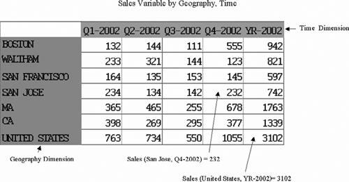
Variable: A variable is used to store data and is equivalent to a fact table in a relational star schema. A variable is defined with respect to a specific set of dimensions. Figure 15.3 shows a conceptual version of how data is stored in a variable. In this example, the sales variable is dimensioned by geography and time. You can query the value of a variable for any values of the dimensions it is defined against. For instance, the sales value for United States for the year 2002 is $3,102. Notice that this is quite like a spreadsheet, where you can retrieve the value of any cell by simply specifying the row and column.
There are several advantages of this multidimensional storage format:
It enforces referential integrity. For instance, if a variable is defined along customer and time dimension, every cell of the data will have some unique value of a customer and time. Also, relationships between dimension values are stored exactly once, and hence you will not end up with inconsistent data such as Boston, MA and Boston, CA.
There is an implicit ordering between rows in the dimension that is defined at creation. This is unlike SQL, where you must explicitly add ORDER BY clauses to return values in a certain order.
Users don’t need to specify how to join the fact and dimension tables to get their answers. They can simply ask to report the variable for any dimension values, as in a spreadsheet. However, unlike a spreadsheet, you are not restricted to two dimensions.
The data is presented to the application as “fully solved.” Once the DBA sets up the analytic workspace with various calculations, the application users do not have to describe how to perform a calculation as part of the query. They just have to indicate which of the available calculations they would like and the calculation engine will take care of the details of computing it. The calculation may be a complex analytical function, a formula, or an aggregate. The data may be precomputed for performance or calculated on the fly; however, the application users do not have to know these details, they simply get the results they ask for.
At this point, you may be wondering what is involved in creating and querying these analytic workspaces. You can use OLAP DML to create dimensions and variables and to load data into the analytic workspace. However, if you would like to use any of Oracle’s tools, such as OLAP API or BI Beans, to manipulate data stored in an analytic workspace, you need to satisfy the following requirements:
You must have a logical model defined in the OLAP Catalog.
The analytic workspace itself must conform to a certain format known as the database standard form.
Sounds like quite a handful! Fortunately, in cases where the data is stored in a relational star or a snowflake schema, such as as the ones described in this book, a simple wizard in Oracle Enterprise Manager can be used to populate the OLAP Catalog from the relational schema. Once you have defined a relational cube in the OLAP Catalog, a wizard in the Analytic Workspace Manager can be used to build the analytic workspace in the standard form.
Hint
The database standard form for an analytic workspace is very complex, and manually creating the analytic workspace elements can be extremely tedious and error prone. It is strongly recommended that you use Analytic Workspace Manager and Oracle Enterprise Manager at least as starting points.
Oracle Database 10g also provides Java APIs to create analytic workspaces. These APIs do not require any preexisting metadata and do not require knowledge of OLAP DML. Due to limitations of space, we will not be discussing these APIs in this book.
In the next sections, as we discuss various other components of Oracle OLAP, we will walk you through the process of defining an analytic workspace from the EASYDW star schema. In section 15.4, we will describe the logical model defined in the OLAP Catalog and populate it using Oracle Enterprise Manager. Then, in section 15.5, we will use the Analytic Workspace Manager tool to create and populate a sample analytic workspace in the standard form. Along the way, we will highlight any assumptions or restrictions imposed by these tools.
Finally, in section 15.6, we will give a brief tour of OLAP DML and illustrate some calculations using the standard form analytic workspace we created. This should help you understand how the multidimensional model can be used to perform analysis instead of, or to complement, the SQL features we have discussed elsewhere in this book.
The OLAP Catalog stores the metadata to specify the logical model for your data. The purpose of defining this metadata is to allow applications to access data using OLAP API or BI Beans. These APIs require that the data is accessible relationally using SQL and require a certain logical metadata model, which we will describe shortly.
The OLAP Catalog metadata can be used regardless of whether your data is in a relational or multi-dimensional format.
If you have a relational schema, the OLAP Catalog simply defines a logical metadata model for this data, as is required by OLAP API and BI Beans. This metadata can also be used to generate a standard form analytic workspace using the Analytic Workspace Manager tool, which we will discuss in section 15.5.
Alternatively, if you have data in a standard form analytic workspace, you can define relational views on top of the multi-dimensional data. The OLAP Catalog can then be defined on these relational views, which can then be used by the OLAP API to access the analytic workspace using SQL. The Analytic Workspace Manager provides wizards to automatically create the required relational views and OLAP Catalog metadata, to enable the analytic workspace for the OLAP API.
Thus, once the requisite metadata has been defined, you can use SQL, OLAP API, or BI Beans to access the data, regardless of whether the data is actually stored in a relational or multidimensional format.
The logical model provided by the OLAP Catalog consists of the following entities:
Dimensions: Dimensions are used to express relationships, such as hierarchies, in your data. Dimensions consist of levels, hierarchies, and level attributes. Note that the SQL dimension object described in Chapter 8 is part of but not the complete metadata for an OLAP Catalog dimension. Also note that the dimension in the OLAP Catalog is not the same as the dimension described in section 15.3.1, which was used to store a list of values in the multidimensional storage format.
Measures: A measure is a quantity that will be used in calculations, such as purchase price or cost.
Measure folders: A measure folder, also known as a measure catalog, is a convenient place to keep related measures together.
Cube: A cube defines how measures will be aggregated across one or more dimensions. In relational terms, it defines how to join your fact and dimension tables. A cube also specifies which hierarchies in the dimensions will be used to compute aggregations.
In the next section, we will discuss how to define OLAP metadata for a relational schema.
OLAP metadata can be defined from a relational schema in two ways:
Using the CWM_OLAP_* and CWM2_OLAP_* packages
Using Oracle Enterprise Manager or Oracle Warehouse Builder tools
The CWM_OLAP_* packages (henceforth referred to as CWM1) are APIs that correspond to the first version of the Common Warehouse Metadata model, also known as CWMLite. This model supports traditional dimension tables, as defined in a star or a snowflake schema. In order to use CWM1 your relational schema must satisfy the following conditions:
The dimension table must be level-based and not parent-child (see Figure 15.2)
If there are multiple hierarchies in a dimension, they must all start with the same base level. Hierarchies where this is not the case, are called ragged hierarchies.
Dimension levels cannot have nulls. Hierarchies where levels can be nulls are called skip-level hierarchies.
The fact table can only have data at the lowest level of the hierarchy. Fact tables where detail data and aggregated data are stored in the same table, known as embedded-total fact tables, are not supported.
A dimension defined using CWM1 in the OLAP Catalog consists of a SQL Dimension object (described in Chapter 8), with some additional descriptive attributes. Oracle Enterprise Manager also provides a graphical user interface to create CWM1 metadata. If you used Oracle Warehouse Builder to design the relational schema for your data warehouse, you can automatically generate metadata from it, according to the CWM1 specification.
The CWM2_OLAP_* packages (henceforth referred to as CWM2) are the second version of CWM1 and provide advanced features not supported by CWM1. If your relational schema has artifacts such as embedded-total fact tables, parent-child dimensions, ragged hierarchies, same value mapping to different levels in different hierarchies, and null values in level columns, you need to use CWM2. At the time of writing, there is no graphical user interface to create this metadata.
Both CWM1 and CWM2 metadata can be viewed in the Analytic Workspace Manager tool.
We will now illustrate the use of Oracle Enterprise Manager to generate OLAP metadata for the EASYDW schema.
You can access the OLAP functionality in Oracle Enterprise Manager from the Administration page (see Chapter 2, Figure 2.16). On this page, in the Warehouse section, you will see links to Cubes, OLAP Dimensions, and Measures, which lead to simple wizards to create and edit dimensions, cubes, and measure folders.
We will define a cube containing the customer, product, and time dimensions using this interface. First, we must define the metadata for the dimensions involved in the cube and then specify the measures and the aggregation operators associated with the cube.
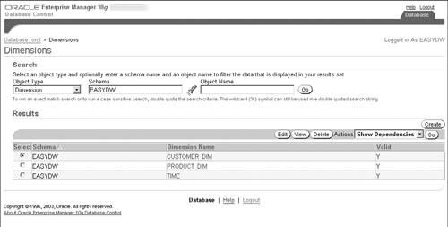
Let us start by going to the OLAP Dimensions page and search for dimensions under schema EASYDW, as shown in Figure 15.4. You will see listed here the SQL Dimension objects we had defined for use with query rewrite in Chapter 9.
To generate the OLAP metadata for a dimension, select the dimension and click on the Edit button. You will get a page similar to the one we discussed in Chapter 8 (Figure 8.5) when creating a dimension—with tabs such as General, Levels, Hierarchies, and Attributes. The last tab is OLAP Options and, when you click on it, you will see a page similar to the one in Figure 15.5. In this figure, we have added OLAP options for the time dimension.
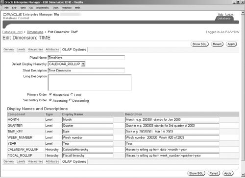
You should now fill in all the descriptive fields on this page, because OLAP API and BI Beans use this information to display various elements related to the dimension. If you press the Show SQL button, you can see the corresponding CWM API calls, as shown in Figure 15.6.

Returning to Figure 15.5, once you press Apply, the CWM metadata will be created. Be assured that your existing SQL dimension object will not be harmed in any way by doing this. Similarly, we can define OLAP metadata for the other two dimensions, Customer and Product. You can now use these dimensions to define your cube objects, as discussed next.
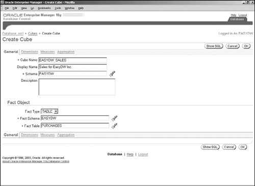
The cube is a metadata object that defines a relationship between the dimensions and measures. From the Administration page (Chapter 2, Figure 2.16), click on the Cubes link to get a page similar to Figure 15.4, except that the Object Type is Cubes. If you press the Create button, you will get the page shown in Figure 15.7. Here, you must specify a name for the cube and the schema where it should reside. You must also indicate the table that would serve as the fact table for this cube. In our example, we are creating the EASYDW_SALES cube using the PURCHASES fact table.
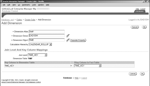
Next, you must click on the Dimensions link and add dimensions to the cube, as shown in Figure 15.8. A cube must have at least one dimension. When adding a dimension to the cube, you must specify how the dimension table joins to the fact table, as well as the default hierarchy to be used to aggregate data along this dimension. In order to do so, after you have entered the dimension name, click the Populate Property button to see the available hierarchies and join key columns, from which you can then choose the ones for the cube. In our example, we have chosen the time dimension, with the hierarchy being CALENDAR_ROLLUP and the join keys being TIME_KEY columns in the dimension and fact tables.
Clicking OK takes you back to the Create Cube page, where you will now see your new dimension in the list. For our example, assume that we have added two more dimensions, CUSTOMER_DIM, and PRODUCT_ DIM to the cube. The next step is to define measures—click the Measures tab and on the next screen click the Add button; you will see the screen as shown in Figure 15.9. This step is easy—you just need to pick the fact table columns that you want to use for analysis.

Click OK to return to the Create Cube page. The final step is to choose the aggregations you would like to perform in this cube—click the Aggregation tab and you will see the page shown in Figure 15.10. Along each dimension, you can pick the aggregation operator from a variety of operators.

As with the dimensions, the Show SQL button allows you to see the CWM APIs to create the cube. Once you have filled in all the information, press OK to create the cube.
Note that none of these operations populates data in the cube. They only define which aggregates are available to an application.
The OLAP metadata can be viewed in several views, such as ALL_OLAP2_CUBES, ALL_OLAP2_DIMENSIONS, and so on.
Once you have defined OLAP metadata created using either Enterprise Manager or CWM2 APIs, it is advisable to validate it and verify access to it. This ensures that the metadata definition is consistent with the underlying schema (i.e., all the tables and columns that the cube refers to exist and the user who created the metadata has access to the data in these tables).
You can check whether a cube or dimension is valid or not in the catalog view, ALL_OLAP2_CUBES, as follows. The INVALID column can have a value Y, N, or O. The value N means that the all the tables, columns, dimension levels, and so on referenced by the cube are present. The value O means that the cube is valid for use by the OLAP API, which means that all additional metadata required by the OLAP API is present. Otherwise, the cube is invalid, which is indicated by the value Y.
SELECT  CUBE_NAME, INVALID FROM ALL_OLAP2_CUBES;

OWNER   CUBE_NAME    INVALID
-----   ------------ -------
EASYDW  EASYDW_SALES O
To validate a cube you must call the CWM2 APIs, as follows, which will validate all underlying dimensions and measures as well. Note that the CWM2_OLAP_MANAGER.SET_ECHO_ON procedure is necessary in order to see the detailed output.
set serveroutput on size 99999
EXECUTE cwm2_olap_manager.set_echo_on;
EXECUTE cwm2_olap_validate.validate_cube
        ('EASYDW','EASYDW_SALES','default','yes'),
The output will indicate if any of the elements of the cube are invalid and the reason will be reported in the COMMENT column (not shown here for lack of space). The third parameter can be default or OLAP API, which will do the basic checks for table and columns or perform additional checks required for using OLAP API. The last parameter indicates whether or not to generate a verbose report.
Validate Cube: EASYDW.EASYDW_SALES
Type of Validation: DEFAULT Verbose Report: YES
Validating Cube Metadata in OLAP Catalog 1
Date: 2004 MAY 21 Time: 22:46:55 User: EASYDW 030922

ENTITY TYPE            ENTITY NAME           STATUS   COMMENT
Cube                   EASYDW.EASYDW_SALES   VALID    ...
  Dimension            EASYDW.CUSTOMER_DIM   VALID
    Hierarchy          CUSTOMER_ZONE         VALID
      Level            CUSTOMER              VALID
        LevelMap                             VALID
        LevelParentMap                       VALID
...
  FactTable            EASYDW.PURCHASES      VALID
    FactLevel          (EASYDW.CUSTOMER_DIM) VALID
    FactLevel          (EASYDW.PRODUCT_DIM)  VALID
    FactLevel          (EASYDW.TIME)         VALID
    FactMeasure        PURCHASE_PRICE        VALID
      FactMeasureMap                         VALID
...
If you plan to use OLAP API or BI Beans directly against the relational schema, you must call the following procedure as the final step after defining the OLAP metadata.
EXECUTE CWM2_OLAP_METADATA_REFRESH.MR_REFRESH;
If you use analytical workspaces, you must instead call the following procedure.
EXECUTE CWM2_OLAP_METADATA_REFRESH.MR_AC_REFRESH;
These procedures are required to populate some underlying cached metadata tables, which are optimized for queries used by the OLAP API.
Finally, you need to verify that the user who created the cube actually has the privileges required to access the underlying tables by using the procedure CWM2_OLAP_VERIFY_ACCESS.VERIFY_CUBE_ACCESS. The parameters of this procedure are the same as those of the VALIDATE_ CUBE procedure.
set serveroutput on size 99999
EXECUTE cwm2_olap_manager.set_echo_on;
EXECUTE CWM2_OLAP_VERIFY_ACCESS.VERIFY_CUBE_ACCESS
        ('EASYDW', 'EASYDW_SALES', 'DEFAULT', 'NO'),
The output of this procedure will appear as follows. Any problems with access are reported in the COMMENT column.
Verify_Cube_Access v_Select_Any_Table:1

***** Verifying User EASYDW access to cube "EASYDW.EASYDW_SALES"
030922.
***** STEP 1: Validate the Cube Metadata.

Validate Cube: EASYDW.EASYDW_SALES Type of Validation: DEFAULT
Verbose Report: NO
Validating Cube Metadata in OLAP Catalog 1
Date: 2004 JULY 02 Time: 01:09:19 User: EASYDW 030922

ENTITY TYPEENTITY NAME STATUS   COMMENT
Cube       EASYDW.EASYDW_SALES    VALID

...

***** STEP 2: Verify the Cached Metadata.
***** STEP 3: Verify Owner.Table.Column access.

***** Validate_Access version 030922 has not found any condition
that would prevent
***** User EASYDW from accessing Cube "EASYDW.EASYDW_SALES".
Note that the procedure will also verify access to the cached metadata created for the OLAP API.
Hint
Always validate the OLAP metadata and refresh the metadata tables after creating or making any changes to it. If it is invalid, the OLAP API and tools may not be able to access the metadata.
Now that we have created the logical model, you can use the Analytic Workspace Manager tool, described next, to create an analytic workspace for this cube.
The Analytic Workspace Manager is a standalone Java application to create, manage, and refresh analytic workspaces. The analytic workspace created by this tool is in a standard form, as required by the Oracle tools. You can also use this tool to enable the analytic workspace for use by OLAP API, BI Beans, and Discoverer.
Hint
The Analytic Workspace Manager application is available on the Oracle Database 10g Client CD. It is not part of Enterprise Manager.
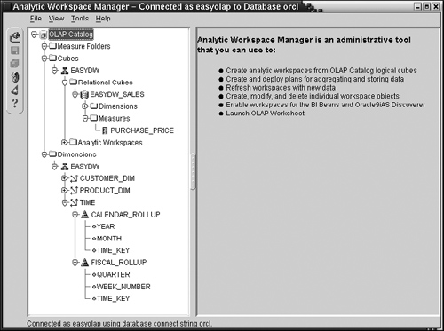
The Analytic Workspace Manager application has two views of the analytic workspaces: the OLAP Catalog View and the Object View. You can switch between the two from the View menu. The OLAP Catalog View shown in Figure 15.11, shows you the OLAP metadata—namely, the dimensions, cubes, and measures that were created using either the CWM1 or CWM2 APIs (or Oracle Enterprise Manager). For instance, in Figure 15.11, we have expanded the view to show the EASYDW_SALES cube and the various dimensions we created earlier.
The Object View, illustrated in Figure 15.12, allows you to browse through various entities in the analytic workspace—namely, dimensions, variables, relations, and so on which we discussed previously.
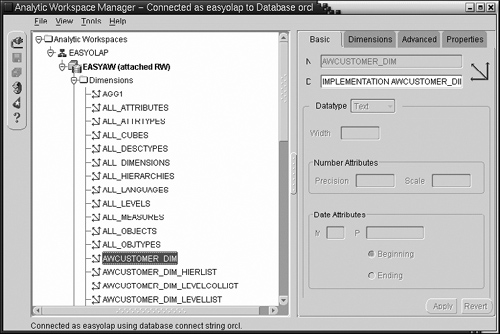
This is a very nifty tool, because the standard form workspace, which we will create shortly, consists of a large number of these entities and it can be very difficult to remember their names.
The Analytic Workspace Manager provides a wizard to create an analytic workspace from a relational cube. You can launch the wizard from the Tools menu, shown in Figure 15.11. We will now use this wizard to create an analytic workspace for the EASYDW_SALES cube.
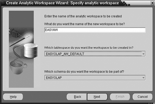
When you launch the wizard, after an introductory page (not shown here), you will see the screen shown in Figure 15.13, where you will be asked to name the analytic workspace, provide a schema where the workspace should be placed, and the tablespace used for storage. It is recommended that you use a different schema to store the analytic workspaces than that used for your relational tables to avoid confusion and potential naming conflicts. The schema owning the analytic workspace must have been granted the OLAP_USER privilege and must have access to the relational tables underlying the cube. Let us assume we have created a new schema, EASYOLAP, and a tablespace, EASYOLAP_AW_DEFAULT, which we will provide here.
When you click the Next button, you will be asked to choose the Cube used to build the analytic workspace, as shown in Figure 15.14.

The next step, shown in Figure 15.15, is to decide whether you would like to load data into the analytic workspace right away or later. Note that the data population stage can take significant time, and in a production system you may want to schedule this at a later time, such as in load window. The Analytic Workspace Manager also includes a wizard to refresh the analytic workspace, discussed in section 15.5.2.

The other option in Figure 15.15 is to generate unique keys for dimension members. Recall that in the multidimensional model, a dimension is just a list of values. So the same value can appear at different levels of the relational dimension table—for example, the name New York could signify either the city or the state. In this case, you may need to qualify the dimension value to distinguish the two levels. If you check the box, the wizard will automatically do this for you.
The next step, shown in Figure 15.16, is to choose an optional naming prefix for the generated objects. In our example, the dimension object PRODUCT_DIM will translate into the dimension AWPRODUCT_DIM in the analytic workspace. It is useful to follow such a naming convention to avoid confusion between relational and multidimensional entities.
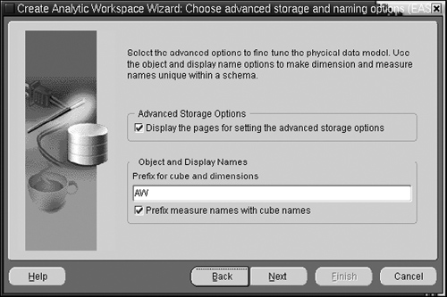
The other option in Figure 15.16 is to decide if you need to change the default storage settings. We will come back to this option in a bit, but for now we will leave it unchecked and accept the d efaults.
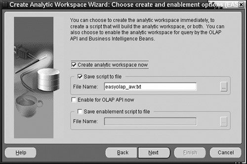
Next, as shown in Figure 15.17, you can decide if you would like to create the analytic workspace immediately or save the script for future use into a file. The script consists of various DBMS_AWM PL/SQL package calls. It can be edited if necessary and executed later in SQL*Plus. You can also choose to enable the analytic workspace for use by OLAP API. This will create several relational views on top of the analytic workspace elements. You can also do this later from the menu.
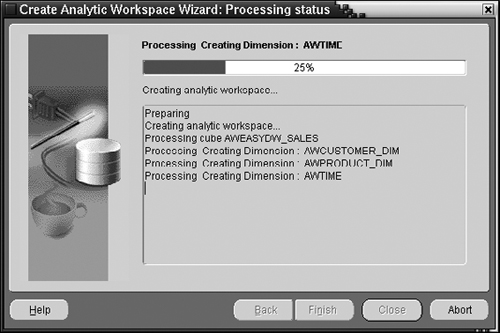
The next screen (not shown here) will give you a chance to review all the options you have chosen. You can then click the Finish button and the wizard will start creating the analytic workspace elements, as shown in Figure 15.18.
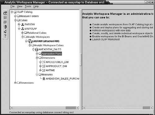
This analytic workspace is now visible under the EASYOLAP schema in the OLAP Catalog View, as shown in Figure 15.19.
Recall that in Figure 15.16, we saw an option to set advanced storage options for the analytic workspace. By default, in an analytic workspace, a variable stores values for every combination of its dimension values. To understand this, recall the conceptual version of a variable that we saw in Figure 15.3. Every cell corresponds to one combination of dimension values. Now, typically, your data may not have entries for every combination—for instance, not every customer buys every product every single day! So we will have a lot of cells with no values, which is a huge waste of space. This problem is addressed by creating a composite dimension. A variable that is dimensioned by a composite dimension will only store values for those combinations of dimension values where data actually exists. This can significantly reduce the space requirements for your analytic workspace.
If there exists data for most values of a dimension, the dimension is said to be dense— otherwise, it is called sparse. By default, the analytic workspace creation wizard assumes that the time dimension is dense and the data across the remaining dimensions is somewhat sparse, specifically that around 30 percent of the dimension combinations have values. Therefore, by default, the wizard creates a composite dimension, which includes all dimensions except the time dimension. If your data does not satisfy these default sparseness assumptions, you can change the default composite dimension or create your own custom composite dimensions.
Hint
For the wizard to detect that a dimension is the time dimension, you would have had to mark it as a time dimension when you created the dimension in the OLAP Catalog.
If you check the box in Figure 15.16, you will get the screen shown in Figure 15.20. Note that composites do add some overhead in processing the queries against the data and hence should not be created unless the data is indeed sparse.
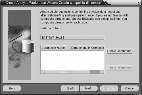
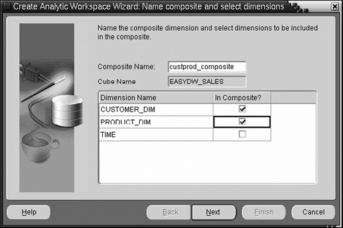
If you press the Create Composite button, you will be taken to the screen shown in Figure 15.21. Now you must give a name to the composite dimension and choose which base dimensions to add to the composite. Typically, you should exclude dense dimensions such as TIME, from the composite.
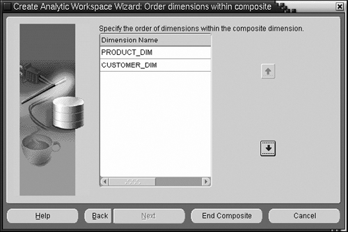
The advanced settings pages also allow you to specify the order of the dimensions for the variable. The order is important, because it affects how data is stored on disk—correctly ordering dimensions within a composite ensures that all data for one value of the composite is clustered together and hence will improve data access performance. Usually, you would want the denser dimensions ahead of the composite and sparser dimensions. For example, if you have transactions for every single day, then the TIME dimension is a dense dimension and should be placed first. Further, on any given day, you would probably have transactions involving most of your products; however, it is less likely you would have transactions involving all your customers. So in this case the product dimension is denser than the customer dimension and should be placed before customers within the composite. The next screen, shown in Figure 15.22, allows you to order the dimensions within the composite.
When you press the End Composite button, your composite will show up in the list in Figure 15.20.
You can choose to group your base dimensions into as many composite dimensions as required by the characteristics of your data. For example, suppose you had five dimensions TIME, PRODUCT, CUSTOMER, GEOGRAPHY, and PROMOTIONS. You may decide to group the CUSTOMER and GEOGRAPHY dimensions together into one composite; since you don’t have all combinations of customers and geographies, the composite will be smaller because it only stores the relevant combinations. Similarly, you can group PRODUCT and PROMOTIONS together into another composite. On the other hand, suppose you wanted to group PRODUCT and GEOGRAPHY into one composite—if you find that you do indeed have transactions for every combination of the two, it would not be advisable to group them into a composite dimension.
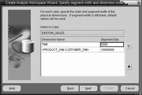
Once you have defined all the composites, when you press the Next button you can now choose the order between various composites and remaining base dimensions, as shown in Figure 15.23. Recall that you must decide the order based on which dimension or composite is denser. In this example, we have placed the denser TIME dimension before the composite. You can also set segment sizes for their storage. In this example, we have specified a segment size of 5KB for the TIME dimension and 10MB for the larger composite dimension.
Once you have done this, you will be back into the normal flow of the wizard, starting in Figure 15.17.
Coming back to the OLAP Catalog View in Figure 15.19, if you right-click on the analytic workspace EASYAW, you will get a menu with several options, as shown in Figure 15.24. From this menu, you can populate the analytic workspace with data from the source tables, which we will discuss next. You can also enable the analytic workspace for Discoverer, OLAP API, and BI Beans, which will be discussed in section 15.5.4.
The Analytic Workspace Manager has a wizard to refresh the analytic workspace from its relational source tables. You must refresh the cubes and dimensions every time there is a change to the source tables that you would like to be visible to the analytic workspace. Note, however, that the refresh process is not incremental and so can take a significant amount of time.
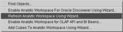
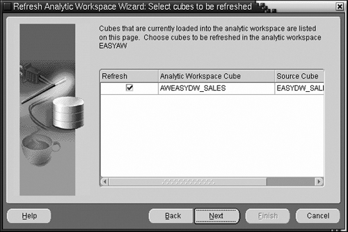
To bring up the refresh wizard, in Figure 15.24, select the Refresh Analytic Workspace Using Wizard option. After the introductory page, you will get the screen shown in Figure 15.25, where you must choose the cube (or cubes) you would like to refresh.
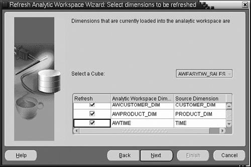
The next step is to choose which dimensions you would like refreshed. In Figure 15.26, we are refreshing all three dimensions. However, note that after initially populating the analytic workspace, you do not need to refresh dimensions unless the underlying dimension tables have changed, which, depending on your business, may be infrequent.
The next button will bring you to a screen (not shown here) similar to Figure 15.17, where you can choose a file to save the script to, if you want to make any customizations to it or execute it later. If you would like the tool to refresh immediately, click the Next button and you will get the screen shown in Figure 15.27, where you can see the refresh of the analytic workspace in progress.

The refresh populates the base-level data into the analytic workspace.
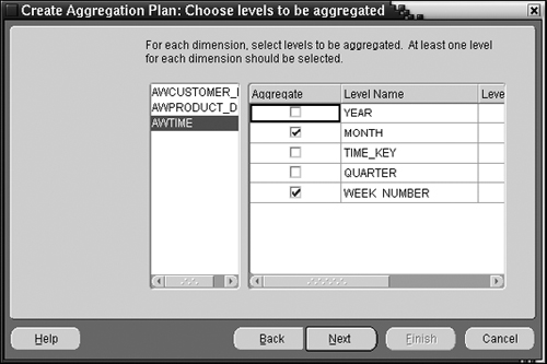
Once you have populated the analytic workspace, you need to create an aggregation plan for this analytic workspace. An aggregation plan or aggregation map determines which levels of the dimension hierarchies you would like to store preaggregated in the analytic workspace. Data at all other levels will be computed on the fly when queries request it. Preaggregated data is analogous to materialized views in the relational world and speeds up queries at the cost of storage space. By striking a good balance between which levels you keep aggregated and which ones you compute on the fly, you can obtain optimal performance within the available storage. One common technique is called skip-level aggregation, where every other level of the cube is preaggregated. We will illustrate this using the wizard in the Analytic Workspace Manager.
If you right-click on the Aggregation Plans node highlighted in Figure 15.19, you will see a popup menu—with one of the options being the wizard to create an aggregation plan. After the customary introduction page, you will be asked to name the aggregation plan (not shown here but assume we have named it AGG1), and then you will see the screen shown in Figure 15.28, where you pick the measures being aggregated.

Note that the aggregation operator used by the wizard is the one you pick when you create the measures in the OLAP Catalog metadata for the source data (see Figure 15.10). The default operator is SUM. To change the aggregation operator after creating the aggregation map, you must issue the following PL/SQL API from SQL*Plus. For example, the following procedure shows how you would change the operator for the purchase price measure to average, along the customer dimension.
EXECUTE DBMS_AWM.SET_AWCUBEAGG_SPEC_AGGOP('AGG1', 'EASYOLAP',
'EASYAW', 'AWEASYDW_SALES', 'AW_EASYDW_SALES_PURCHASE_PRICE',
'AWCUSTOMER_DIM', 'AVERAGE'),
The next step, shown in Figure 15.29, allows you to choose which levels should be aggregated for each dimension. In this example, we are doing a skip-level aggregation by aggregating every other level in each hierarchy (i.e., in the fiscal rollup hierarchy we are aggregating at the WEEK_NUMBER level and in the calendar rollup, we are aggregating at the MONTH level).
Once you click the Next button, you get to review the choices you have made, as shown in Figure 15.30. Clicking the Finish button creates the aggregation plan. Note that the aggregates are not actually built until you deploy the aggregation plan.

To deploy the aggregation plan, right-click on the desired aggregation plan node in the OLAP Catalog View (Figure 15.11) and choose menu item Deploy aggregation plan using wizard. This is a simple one-page wizard, which will ask for confirmation and then start the aggregation process to compute the levels specified by the plan.
The Analytic Workspace Manager provides enablers to adapt the analytic workspace for Discoverer and OLAP API. The enablers are simple wizards and can be launched from the menu shown in Figure 15.24.
The enabler for OLAP API and BI Beans is very simple (looks like Figure 15.17) and simply produces the required relational views that allow the API to access the multidimensional data. You can also save the script to a file to be executed later.
In Chapter 13, we saw how to use Discoverer for adhoc querying and reporting for endusers who may not know SQL. You can use Discoverer to query your multi-dimensional data as well. The Analytic Workspace Manager provides a wizard that will adapt the analytic workspace to work with Discoverer.
The wizard produces two items:
A SQL script, which contains the relational views that Discoverer needs to access the data in the analytic workspace. This must be run from SQL*Plus.
An EEX file, which has an XML script to build an EUL layer. This should be imported into Discoverer using the Administrator, discussed in Chapter 13.
Once you have done this, you can start using Discoverer to access the data.
Hint
If you make any metadata changes to the analytic workspace or the OLAP Catalog, such as adding a new dimension, cube, or measure, you must rerun the enablers.
Now that we have built an analytic workspace in standard form, we will illustrate how analysis can be done on this workspace.
Oracle OLAP provides several ways by which an application can access multidimensional data in an analytic workspace. These are shown in Figure 15.31.
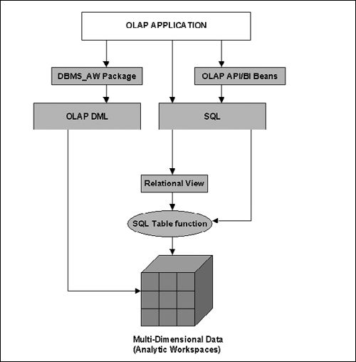
The primary language to access analytic workspaces is OLAP DML. OLAP DML is a very simple but powerful language that allows you to express a variety of calculations and do spreadsheet-like reporting on data stored in an analytic workspace. It provides functions for forecasting, allocation, aggregation, statistical analysis, and financial calculations. You can execute OLAP DML using the OLAP Worksheet application (described in section 15.6.1) or in the Analytic Workspace Manager.
Java programs can access analytic workspaces using the OLAP API, provided that appropriate OLAP Catalog metadata has been defined. SQL applications can access the data by defining Table Functions that convert the data into rows. Relational views may be defined on top of the Table functions, so that the application does not know whether the underlying data is stored in analytic workspaces or tables.
We will now discuss each of these mechanisms in some detail.
Figure 15.32 shows the OLAP Worksheet application, which is a simple application (like SQL*Plus) that allows you to execute OLAP DML commands. You can launch the OLAP Worksheet from the command line using the standalone executable called wrksht on UNIX or wrksht.bat on Windows. You can also launch it from the Tools menu in the Analytic Workspace Manager application. You issue the OLAP DML commands in the lower portion of the window and the results appear in the upper portion.
Hint
OLAP DML is very different and completely separate from SQL. However, there is a SQL mode in the OLAP Worksheet, where you can issue regular SQL statements as in SQL*Plus. Conversely, you can issue OLAP DML commands in SQL*Plus using the DBMS_AW package, described in section 15.6.2.
One thing to bear in mind is that OLAP Worksheet is not a graphical user interface to query the analytic workspace. It only allows you to enter OLAP DML commands. In other words, you must know OLAP DML to use this tool. However, the OLAP Worksheet has an excellent help system, which describes all OLAP DML commands with examples. In the next few sections, we will show some examples of using OLAP DML to illustrate the types of calculations that can be done with analytic workspaces. Note that this is not a tutorial on OLAP DML and we will not go into details of OLAP DML syntax.
Before you can access the analytic workspace, you must first attach to an analytic workspace using the AW ATTACH OLAP DML command. The examples in the following sections will use the analytic workspace, named EASYAW, that we created earlier using the Analytic Workspace Manager tool.
Hint
In the following examples, the OLAP DML command is prefixed with the prompt -> and followed by its output.
To attach to the EASYAW analytic workspace, issue the following OLAP DML command in the OLAP Worksheet tool. The readwrite keyword allows you to save changes to the workspace:
-> aw attach easyaw readwrite
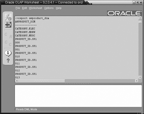
Once this command returns successfully, you can then issue other OLAP DML commands to access the analytic workspace—for instance, in Figure 15.32, we are querying a dimension named AWPRODUCT_DIM.
The analytic workspace EASYAW, created using the Analytic Workspace Manager, is in a special format called the database standard form, which consists of several dimensions and relations that describe the structure of the analytic workspace. You can browse through all of these in the Object View in the Analytic Workspace Manager, shown earlier in Figure 15.12. To see the definition of any entity in OLAP DML, right-click on it to bring up a popup menu and choose the View Details option.
Alternatively, you can issue the FULLDSC command from the OLAP Worksheet. For instance, the AWTIME dimension will appear as follows:
-> FULLDSC AWTIME

DEFINE AWTIME DIMENSION TEXT
LD IMPLEMENTATION AWTIME Dimension
PROPERTY 'AW$CLASS' - 'IMPLEMENTATION'
PROPERTY 'AW$CREATEDBY' - 'AW$CREATE'
PROPERTY 'AW$LASTMODIFIED' -'20MAY04_16:23:32'
PROPERTY 'AW$LOGICAL_NAME' - 'AWTIME'
...
The various properties are part of the standard form definition and you would not ordinarily need to know the details of these.
Another example of a standard form entity is the variable AWEASYDW_ PURCHASE_PRICE_VARIABLE, which was derived from the measure PURCHASE_PRICE in the OLAP Catalog. Its definition is as follows:
-> FULLDSC AWEASYDW_SALES_PURCHASE_PRICE_VARIABLE

DEFINE AWEASYDW_SALES_PURCHASE_PRICE_VARIABLE
VARIABLE DECIMAL
<AWEASYDW_SALES_COMPOSITE <AWCUSTOMER_DIM AWPRODUCT_DIM AWTIME>>
The items in the angle brackets are the dimensions along which the variable is defined. Notice that a composite dimension has been defined to include all the base dimensions.
We will see more standard form entities in the next section.
Previously, we described various entities in an analytic workspace, such as dimensions, relations, and variables. The REPORT command can be used to query data in these entities. When reporting data in a dimension, the report command produces the list of values in the dimension. When reporting data in a variable, the report command returns the answer like a spreadsheet, typically with one dimension along the rows and another along the columns.
For example, one of the entities in the EASYAW analytic workspace is the AWTIME dimension. The following command reports the values of the AWTIME dimension. Notice how values at different levels in a hierarchy are all part of the same dimension.
-> report awtime

AWTIME
--------------
MONTH.200301
MONTH.200302
...
TIME_KEY.01-JAN-03
TIME_KEY.02-JAN-03
...
YEAR.2003
YEAR.2004
...
In the next example, we are querying the AWTIME_LEVELREL relation. This is a standard form relation, which maintains the relationship between each value in a dimension and the level it corresponds to. For example, the value MONTH.200301 corresponds to the MONTH level and the value YEAR.2003 corresponds to the YEAR level.
-> report down awtime awtime_levelrel

AWTIME                           AWTIME_LEVELREL
------------------------------ --------------------
MONTH.200301                   MONTH
MONTH.200302                   MONTH
...
TIME_KEY.23-DEC-04             TIME_KEY
TIME_KEY.24-DEC-04             TIME_KEY
...
YEAR.2003                      YEAR
YEAR.2004                      YEAR
...
At this point, you may find it to be a worthwhile exercise to try similar report commands on some of the other dimensions and relations in the EASYAW analytic workspace. Remember that you can browse the various entities in the Object View of the Analytic Workspace Manager in Figure 15.12.
You can restrict the data you are querying to a specific value or list of values using the LIMIT command. This is similar to a selection specified by a WHERE clause in SQL. However, unlike SQL, where the selection is specified on a per query basis, the limit commands in an OLAP DML persist as long as you are attached to the analytic workspace. The next example limits the AWTIME dimension to only those values that have the AWTIME_LEVELREL value of MONTH.
-> LIMIT awtime to awtime_levelrel EQ 'MONTH'
-> REPORT awtime

AWTIME
------------------------------
MONTH.200301
MONTH.200302
MONTH.200303
...
Now we get to the more interesting part about reporting data from a variable. The OLAP analysis engine automatically figures out the dimensions involved, using the definition of the variable. The keyword ACROSS indicates that the AWTIME dimension values will be reported along the row. The engine then automatically places the other dimensions in the report. In the following example, we are reporting sales by state for January through June 2003 for the HDRW product category.
-> LIMIT awcustomer_dim TO awcustomer_dim_levelrel EQ 'STATE'
-> LIMIT awtime TO 'MONTH.200301' TO 'MONTH.200303'
-> LIMIT awproduct_dim TO 'CATEGORY.HDRW'
-> REPORT across awtime : aweasydw_sales_purchase_price_variable

AWPRODUCT_DIM: CATEGORY.HDRW
                               AWEASYDW_SALES_PURCHASE_PRICE_VA
                               -------------RIABLE-------------
                               -------------AWTIME-------------
                               MONTH.2003 MONTH.2003 MONTH.2003
AWCUSTOMER_DIM                     01         02         03
------------------------------ ---------- ---------- ----------
STATE.AZ                           501.44     391.75     376.08
STATE.CA                           407.42     391.75     297.73
STATE.CT                           501.44     329.07     407.42
STATE.IL                           454.43     376.08     360.41
...
STATE.OH                           376.08     329.07     329.07
STATE.TX                           376.08     282.06     297.73
STATE.WA                           391.75     360.41     282.06
You may be wondering how we were automatically able to generate sales data at a MONTH level without specifying any aggregation functions like SUM, to rollup from the detail data. Recall that in section 15.5.3, after populating the analytic workspace, we created an aggregation plan, which indicated the levels for which to pre-aggregate data in the variable. When creating this plan, we had specified that the MONTH and STATE levels be pre-aggregated and hence we could report along these levels automatically. This is in fact one of the most powerful features of the multi-dimensional model, which differentiates it from SQL.
For levels that were not preaggregated, the aggregation can be performed on the fly by using the AGGREGATE function and specifying the aggregation map. In the following example, we are limiting the customer dimension to the REGION level (which was not precomputed), the product dimension to the HDRW category, and the months to January–March 2003; we are using the aggregation plan AWEASYDW_SALES_AGGMAP_AGG1 to compute the total sales.
-> LIMIT AWCUSTOMER_DIM TO AWCUSTOMER_DIM_LEVELREL EQ 'REGION'
-> LIMIT AWPRODUCT_DIM TO 'CATEGORY.HDRW'
-> LIMIT AWTIME TO 'MONTH.200301' TO 'MONTH.200303'

-> REPORT across AWTIME:
   AGGREGATE(aweasydw_sales_purchase_price_variable USING
             aweasydw_sales_aggmap_agg1)

AWPRODUCT_DIM: CATEGORY.HDRW
                               AGGREGATE(AWEASYDW_SALES_PURCHAS
                               -----E_PRICE_VARIABLE USING-----
                               --AWEASYDW_SALES_AGGMAP_AGG1)---
                               -------------AWTIME-------------
                               MONTH.2003 MONTH.2003 MONTH.2003
AWCUSTOMER_DIM                     01         02         03
------------------------------ ---------- ---------- ----------
REGION.AmerMidWest                 830.51     705.15      689.48
REGION.AmerNorthEast             1,817.72   1,378.96    1,629.68
REGION.AmerNorthWest               391.75     360.41      282.06
REGION.AmerSouth                   376.08     282.06      297.73
REGION.AmerWest                    908.86     783.50      673.81
REGION.EuroWest                  2,146.79   1,755.04    1,786.38
Instead of having end users specifying the aggregation function every time they query, the DBA can set the aggregation plan as a default for a variable, as follows:
-> AGGMAP SET aweasydw_sales_aggmap_agg1 AS DEFAULT FOR
              aweasydw_sales_ship_charge_variable
Now, every time the end users do a report command, the aggregation will be automatically returned, either by computing it on the fly or by using the precomputed values. This is illustrated in the following example, where we report on the AWEASYDW_SALES_SHIP_CHARGE_VARIABLE.
-> REPORT ACROSS awtime: aweasydw_sales_ship_charge_variable

                              AWEASYDW_SALES_SHIP_CHARGE_VARIA
                              --------------BLE---------------
                              -------------AWTIME-------------
                              MONTH.2003 MONTH.2003 MONTH.2003

AWCUSTOMER_DIM                       01         02         03
------------------------------   ----------  ---------  ---------
REGION.AmerMidWest                   238.50     202.50     198.00
REGION.AmerNorthEast                 522.00     396.00     468.00
REGION.AmerNorthWest                 112.50     103.50      81.00
REGION.AmerSouth                     108.00      81.00      85.50
REGION.AmerWest                      261.00     225.00     193.50
REGION.EuroWest                      616.50     504.00     513.00
Here you can see simplicity and the power of the multidimensional model—we do not need to specify the join, aggregation, or repeat the clauses as in SQL!
You can also compute other variables using the variables defined earlier. For instance, the following example defines a variable named AWEASYDW_ TOTAL_SALES_VARIABLE and computes it using the sum of two other variables.
-> DEFINE AWEASYDW_TOTAL_SALES_VARIABLE
-> VARIABLE DECIMAL
   <AWEASYDW_SALES_COMPOSITE
             <AWCUSTOMER_DIM AWPRODUCT_DIM AWTIME>>

-> LIMIT awtime TO awtime_levelrel EQ 'QUARTER'
-> LIMIT awcustomer_dim TO awcustomer_dim_levelrel EQ 'STATE'
-> LIMIT awproduct_dim TO awproduct_dim_levelrel EQ 'CATEGORY'

-> ACROSS awtime awcustomer_dim awproduct_dim
   DO 'aweasydw_total_sales_variable =
       aweasydw_sales_purchase_price_variable +
       aweasydw_sales_ship_charge_variable'
The ACROSS DO construct in the preceding example loops over the values in each of the dimensions, as specified by the limit clauses, and performs the computation for each value combination. We can now use it to report the variable, as in the following example. Here, we also illustrate another standard form construct, the PARENTREL relation. This relation maintains the relationship between a value and its parent value in a given dimension hierarchy. We limit the AWCUSTOMER_DIM dimension to those values (states) whose parent (region) is the AmerNorthEast region.
-> LIMIT awtime TO awtime_levelrel EQ 'QUARTER'
-> LIMIT AWCUSTOMER_DIM TO AWCUSTOMER_DIM_PARENTREL EQ
                          'REGION.AmerNorthEast'
-> LIMIT AWPRODUCT_DIM TO 'CATEGOR.HDRW'

-> REPORT DOWN awtime ACROSS awcustomer_dim:
               aweasydw_total_sales_variable

AWPRODUCT_DIM: CATEGORY.HDRW
               -------AWEASYDW_TOTAL_SALES_VARIABLE-------
               --------------AWCUSTOMER_DIM---------------
AWTIME          STATE.CT   STATE.MA   STATE.NH   STATE.NY
-------------- ---------- ---------- ---------- ----------
QUARTER.200301   1,593.43   1,593.43   1,311.05   1,573.26
QUARTER.200302   1,694.28   1,835.47   1,532.92   1,754.79
QUARTER.200303   1,714.45   1,734.62   1,311.05   1,593.43
QUARTER.200304   1,734.62   1,875.81   1,391.73   1,633.77
...
With OLAP DML you can also define formulas to perform calculations using simple arithmetic or analytic functions. Once defined, users can then reference these calculations in reports like any other variables defined earlier. We should emphasize that the end user does not need to know how the calculation was done or which analytic function it used.
The next example creates a formula to determine difference in sales between the current month and the previous month using the LAGDIF function. This function is similar to the LAG SQL analytic function we saw in Chapter 6, except that it returns the difference between the current value and the value at the specified LAG offset. The LAGDIF function in OLAP DML takes as arguments a variable name, the LAG offset, a dimension along which to compute the LAG, and an optional LIMIT command, which can be used to restrict the values of the dimension. In this example, we are using the AWEASYDW_SALES_PURCHASE_PRICE_VARIABLE, along the AWTIME dimension. The LIMIT command restricts the computation to only the month level and the LAG offset is 1—in other words, the previous month.
-> DEFINE AWEASYDW_SALES_PREV_MONTH
   FORMULA
   DECIMAL <AWCUSTOMER_DIM AWPRODUCT_DIM AWTIME>
   EQ LAGDIF (AWEASYDW_SALES_PURCHASE_PRICE_VARIABLE,1,
              AWTIME, AWTIME_LEVELREL EQ 'MONTH')

-> LIMIT awproduct_dim TO 'CATEGORY.HDRW'
-> LIMIT awcustomer_dim TO 'REGION.AmerNorthEast'
-> LIMIT awtime TO awtime_levelrel EQ 'MONTH'
We can now use this formula to report the sales for the current month and the difference between the sales for the current and the previous month.
-> REPORT down awtime across awproduct_dim:
   <AWEASYDW_SALES_PURCHASE_PRICE_VARIABLE,
    AWEASYDW_SALES_PREV_MONTH>

AWCUSTOMER_DIM: REGION.AmerNorthEast
                     ----AWPRODUCT_DIM----
                     ----CATEGORY.HDRW----
                     AWEASYDW_S
                     ALES_PURCH AWEASYDW_S
                     ASE_PRICE_ ALES_PREV_

AWTIME                VARIABLE    MONTH
-------------------- ---------- ----------
MONTH.200301           1,817.72         NA
MONTH.200302           1,378.96    -438.76
MONTH.200303           1,629.68     250.72
MONTH.200304           1,817.72     188.04
MONTH.200305           1,896.07      78.35
...
So far all the examples we have seen could also have been performed with SQL. The following section illustrates one of the advanced features of the OLAP Engine that is currently not available in SQL: forecasting.
One of the common operations performed using OLAP DML is forecasting. To forecast a quantity such as sales we must perform the following steps:
Define variables to store the forecast results.
Specify the parameters of the forecast.
Execute the forecast.
We will show a very simple example of forecasting future sales based on historical sales.
The first step is to define a variable called AWEASYDW_SALES_ FORECAST_VARIABLE, which stores the result of the forecast. Note again that we have dimensioned this variable just like the AWEASYDW_SALES_PURCHASE_PRICE_VARIABLE.
-> DEFINE AWEASYDW_SALES_FORECAST_VARIABLE VARIABLE DECIMAL
   <AWEASYDW_SALES_COMPOSITE
                  <AWCUSTOMER_DIM AWPRODUCT_DIM AWTIME>>
Next, we constrain the AWTIME dimension to the month level and customers to customer id level. This means that the forecast will be computed using the months in the AWTIME dimension for each customer id value in the AWCUSTOMER_DIM dimension.
-> LIMIT AWTIME TO AWTIME_LEVELREL EQ 'MONTH'
-> LIMIT AWCUSTOMER_DIM TO AWCUSTOMER_DIM_LEVELREL EQ 'CUSTOMER'
-> LIMIT AWPRODUCT_DIM TO 'CATEGORY.HDRW'
To specify parameters and run the forecast, we must create a handle, which will be used by subsequent commands. The handle, called sf_handle, is obtained by calling the FCOPEN command to which you specify a name.
-> DEFINE sf_handle VARIABLE INTEGER;

-> sf_handle = FCOPEN('EasyDWSalesForecast')
Next, we will set the forecast parameters using the FCSET command. We are using the automatic method for forecasting. We will consider three time periods (months) as historical data and forecast using a periodicity parameter of 6, which indicates the interval over which the sales repeat.
-> FCSET sf_handle method 'automatic' histperiods 3 periodicity 6
Finally, we execute the forecast using the FCEXEC command. We must specify the name of the time dimension and also the variable containing the data to be used for the forecast—in our case, AWEASYDW_SALES_PURCHASE_PRICE_VARIABLE. The results are placed into the AWEASYDW_SALES_SALES_ FORECAST_VARIABLE we defined earlier.
-> FCEXEC sf_handle TIME AWTIME
   INTO AWEASYDW_SALES_FORECAST_VARIABLE
   AWEASYDW_SALES_PURCHASE_PRICE_VARIABLE
Finally, we close the handle as follows:
-> FCCLOSE sf_handle
You can now query this variable to forecast the sales. You can also use an aggregation map to aggregate the forecast to higher levels. In the following example, we are forecasting sales for January 2005 for customers in Massachusetts (STATE.MA).
-> LIMIT awtime to 'MONTH.200501'
-> LIMIT awcustomer_dim to awcustomer_dim_parentrel eq 'STATE.MA'
-> LIMIT AWPRODUCT_DIM TO 'CATEGORY.HDRW'

-> REPORT down awcustomer_dim across awtime:
               AWEASYDW_SALES_FORECAST_VARIABLE

AWPRODUCT_DIM: CATEGORY.HDRW
                               AWEASYDW_S
                               ALES_FOREC
                               AST_VARIAB
                               ----LE----
                               --AWTIME--
                               MONTH.2005
AWCUSTOMER_DIM                     01
------------------------------ ----------
CUSTOMER.AB123410                   31.34
CUSTOMER.AB123420                   15.67
CUSTOMER.AB123440                    0.00
CUSTOMER.AB123450                    0.00
...
CUSTOMER.AB123500                    9.25
CUSTOMER.AB123510                   13.93
CUSTOMER.AB123530                   22.63
CUSTOMER.AB123540                   24.38
...
In this section, we have given you a quick but broad overview of OLAP DML and analytic workspaces. We saw how data is stored, aggregated, calculated, and reported in the multidimensional format. We have only scratched the surface of what can be done with OLAP DML, but hopefully you have gotten some idea of the simplicity and power of this language.
Besides interactively issuing OLAP DML using the OLAP Worksheet, you can also use it within an application, as discussed in the next section.
The DBMS_AW package provides functions that allow you to execute OLAP DML commands and programs using PL/SQL programs or SQL*Plus.
The EXECUTE procedure can be used to execute one or more OLAP DML commands and print the output to the screen using the DBMS_OUTPUT package. The following example attaches to the EASYAW analytic workspace and reports the dimension AWTIME.
SET SERVEROUTPUT ON;
BEGIN
  DBMS_AW.EXECUTE(q'[
  AW ATTACH easyaw
  LIMIT awtime to awtime_levelrel EQ 'MONTH'
  REPORT awtime
  AW DETACH easyaw
]'),
END;
/

AWTIME
--------------
MONTH.200301
MONTH.200302
MONTH.200303
MONTH.200304
MONTH.200305
MONTH.200306
MONTH.200307
...
PL/SQL procedure successfully completed.
Applications can access multidimensional data stored in analytic workspaces with SQL by using SQL Table functions. Oracle provides a table function called OLAP_TABLE to do this, but you can also write your own custom table functions.
The OLAP_TABLE function takes four parameters:
The analytic workspace to attach to. You can specify whether to attach the workspace for a query or for a session.
An optional type for the result of the OLAP_TABLE function. Recall from Chapter 5 that a table function is similar to a table and returns rows as its result. So you must first define a type for the rows being returned and a type for the table. This parameter is useful if you would like to control the data types returned. If not specified, the results are converted to SQL data types.
This parameter allows you to specify any OLAP command. A common use of this parameter involves specifying OLAP DML FETCH commands, which indicate how to fetch data from the analytic workspace. It is usually omitted and the next parameter, called the limit map is used instead. If specified, this command is executed prior to the limit map.
The last parameter is called the LIMIT MAP and specifies how data in the analytic workspace maps to columns in the table returned by the OLAP_TABLE function. The limit map defines measures, dimensions, and their hierarchies. When the OLAP_TABLE function is used in a SQL query, the limit map, in combination with the SQL WHERE clause, will issue OLAP DML LIMIT commands to the analytic workspace to restrict data returned.
We will explain these with the following example, which retrieves the data from the variable AWEASYDW_PURCHASE_PRICE_VARIABLE in the EASYAW analytic workspace. We will define a TYPE, named PURCHASES_TYPE, which describes the rows being returned, and a TYPE, named PURCHASE_TABLE, which describes the table of these rows. For each dimension, we will return the value and the GROUPING_ID function, which indicates the level the value corresponds to (see Chapter 6 for a description of the GROUPING_ID SQL function).
CREATE TYPE purchases_type AS OBJECT
(cust VARCHAR2(80),
 cust_gid NUMBER,
 time VARCHAR2(30),
 time_gid NUMBER,
 prod VARCHAR2(30),
 prod_gid NUMBER,
 purchase_price NUMBER);
/
Next, we define a type, PURCHASE_PRICE_TYPE, which describes a table whose rows are of the PURCHASE_TYPE:
CREATE TYPE purchases_table AS TABLE OF purchases_type;
/
We will define a relational view on the table function as follows, so that applications can access this data without really needing to know about table functions and OLAP DML.
CREATE VIEW purchase_price_view
as
SELECT * FROM TABLE(OLAP_TABLE(
'easyaw duration session', 'purchases_table', '',
'dimension cust from awcustomer_dim
  with hierarchy awcustomer_dim_parentrel
  gid cust_gid from awcustomer_dim_gid
 dimension time from awtime
  with hierarchy awtime_parentrel
  gid time_gid from awtime_gid
 dimension prod from awproduct_dim
  with hierarchy awproduct_dim_parentrel
  gid prod_gid from awproduct_dim_gid
 measure purchase_price
  from aweasydw_sales_purchase_price_variable
'));
This view is now queried like any other relational table. For instance, in the following example, we are querying hardware sales in Massachusetts.
SELECT time, sum(purchase_price)
FROM purchase_price_view
WHERE prod = 'CATEGORY.HDRW' and cust = 'STATE.MA'
GROUP BY time

TIME                           SUM(PURCHASE_PRICE)
------------------------------ -------------------
MONTH.200301                                 470.1
MONTH.200302                                360.41
...
QUARTER.200402                             1284.94
QUARTER.200403                             1300.61
...
YEAR.2003                                  5468.83
...
Note that when you enable the analytic workspace for OLAP API using the analytic workspace manager, the relational views created by the tool use the OLAP_TABLE function.
Thus, using table functions and relational views, the OLAP DML commands can be completely hidden away, and the SQL application can now be completely unaware of whether the data being accessed is stored in a relational or a multidimensional format.
The OLAP API is a set of Java classes that can be used to develop OLAP applications. It is very well suited to developing thin-client applications that can be accessed with a Web-browser. The OLAP API uses a multidimensional model for querying data; however, it internally translates these queries into SQL. To access objects using this API, you need to have defined the objects in the OLAP Catalog. The underlying data may be stored either in relational tables or in analytic workspaces encapsulated within relational views.
Business Intelligence Beans (BI Beans) is a set of reusable components that allows you to rapidly develop OLAP applications. They are integrated into Oracle’s JDeveloper product, where they can be created and customized using simple wizards. BI Beans can perform a wide range of tasks, such as connecting to a database, building queries to perform analytical calculations, and displaying the results in extremely powerful reports, tables, or graphs. These components can then be easily deployed as part of a Java or JSP application.
A novel aspect of BI Beans is that you have full access to the data as the component is being designed, so you can immediately see how the resulting graph or presentation will look. Before you start to build business intelligence components, you must set up a database connection using the Designer bean. Then you can use the Query Builder to define queries, Presentation Wizard to create a report or graph, and Calculation Builder to define calculations.
A detailed discussion of the OLAP APIs and BI Beans is beyond the scope of this book.
In this chapter, we have seen how Oracle can be used to perform multidimensional analysis using the Oracle OLAP option. The multidimensional model is an intuitive model for analysis, because the application does not need to know how to join fact tables with dimension tables or to express analytic functions using SQL. Analytic workspaces provide a way to store and preaggregate data in a multidimensional format. The OLAP calculation engine provides several advanced features, such as forecasting and allocation, that are not available in SQL. You can map the analytic workspace back to a relational model for use by OLAP API and BI Beans applications by defining relational views on top of it. The Analytic Workspace Manager tool simplifies creation and maintenance of analytic workspaces from a relational star or snowflake schema and also provides wizards to automatically create the views required for the analytic workspace to be used by applications such as Discoverer or BI Beans.
Thus, regardless of whether you store your data in relational or multidimensional format, the Oracle database provides all the tools and techniques required for advanced business analysis applications.
In the next chapter, we will discuss another technique for business analysis—data mining, which can be used to determine hidden trends and patterns in your data.