
Chapter 11
PEEC Models for Magnetic Material
11.1 Inclusion of Problems with Magnetic Materials
Models with magnetic materials can be a part of many different interesting PEEC solutions. This leads to a different class of issues. In some structures, magnetic bodies may be a small part of the overall problem. Examples are a small inductor on a chip, a filter on a printed circuit board (PCB), or a microwave filter. On the other hand, substantial parts of a problem can consist of magnetic materials. Other examples are parts of a motor or a very large transformer. Different solution approaches are necessary to cover such a wide range of problems. Hence, different models may be used to include magnetic materials in partial element equivalent circuit (PEEC) models.
The first approach considered in Section 11.1 deals with magnetically closed loops such that the magnetic part may be treated separately from the rest of the problem. For this class of problems, the solution may result in a simpler model. We consider how such a model is applied in a PEEC environment. In fact, integrating such a part may be very simple since it can be included as circuit models. The second class of problems consists predominantly of magnetic materials, where most of the solution is based on magnetic materials.
11.1.1 Magnetic Circuits for Closed Flux Type Class of Problems
We first consider perhaps one of the oldest solution methods for magnetic problems, which was and still is applied, including many situations such as power electronics problems and transformers or motors, for example, [1, 2]. The key assumption is that the majority of the magnetic flux is in the magnetic material rather than through the air. Today, this class of problems can also include chokes used with PCBs as well as other magnetic core structures such as magnetic memory cores. An interesting aspect is that we can solve this class of problems by using a circuit analog. To compare the corresponding statement for the electrical and magnetic circuits, we display the electrical circuit equation on the left and the equivalent magnetic one on the right side in the derivation.
We first show in Fig. 11.1 part of a magnetic circuit to define the geometrical parameters such as the cross section ![]() and the length
and the length ![]() . However, we should remark that the reluctance approach does not work well for open-loop problems such as the bar shown in Fig. 11.1. Hence, we assume that it is a portion of a loop without large gaps.
. However, we should remark that the reluctance approach does not work well for open-loop problems such as the bar shown in Fig. 11.1. Hence, we assume that it is a portion of a loop without large gaps.

Figure 11.1 Simple example bar of magnetic material.
Corresponding to the electrical potential, we define an artificial magnetic potential ![]() with the integral form
with the integral form

![]() and
and ![]() are the line integration starting position and the ending position respectively. The relationship between the current density and electrical fields is in terms of the conductivity
are the line integration starting position and the ending position respectively. The relationship between the current density and electrical fields is in terms of the conductivity ![]() for conductors that corresponds to the permeability
for conductors that corresponds to the permeability ![]() in the magnetic material.
in the magnetic material.
The relation between current and current density corresponds to the magnetic field and the magnetic flux

where ![]() is the electrical current and
is the electrical current and ![]() is the magnetic flux in the magnetic equivalent circuit. It is equivalent to the electrical current for electrical circuits.
is the magnetic flux in the magnetic equivalent circuit. It is equivalent to the electrical current for electrical circuits.
In this case, we use the current flow type notation ![]() for the area on purpose for the magnetic flux since it corresponds to the current in the conventional circuit case. Again,
for the area on purpose for the magnetic flux since it corresponds to the current in the conventional circuit case. Again, ![]() corresponds to current and
corresponds to current and ![]() corresponds to current density. With this, Ohm's law with the reluctance resistance corresponds to
corresponds to current density. With this, Ohm's law with the reluctance resistance corresponds to
Finally, we see a difference between the quasistatic equations for the electrical and magnetic fields where

By comparing (11.2) and (11.7), we find for the closed loop that
where ![]() is the total current penetrating the loop. We see that the magnetic equivalent circuit equation differs in an important way in that the closed loop in (11.7) leads to an equivalent voltage source corresponding to the driving voltage. This requires some adjustment in thinking. Notethat the units of the magnetic potential is A or Amperes. We need to note that the current
is the total current penetrating the loop. We see that the magnetic equivalent circuit equation differs in an important way in that the closed loop in (11.7) leads to an equivalent voltage source corresponding to the driving voltage. This requires some adjustment in thinking. Notethat the units of the magnetic potential is A or Amperes. We need to note that the current ![]() is the total conventional current. We see that for a multiturn loop with
is the total conventional current. We see that for a multiturn loop with ![]() -turns, the current may be entering the loop
-turns, the current may be entering the loop ![]() times, which results in an
times, which results in an ![]() multiplication to get the total contributing current. The first equation of (11.7) results from Faraday's law and the second equation in (11.7) is the well-known Ampere's law.
multiplication to get the total contributing current. The first equation of (11.7) results from Faraday's law and the second equation in (11.7) is the well-known Ampere's law.

Figure 11.2 Magnetic transformer core example.
11.1.2 Example for Inductance Computation
First, we apply the equivalent magnetic circuit Ohm's law equation (11.6) to an example of a magnetic core shown in Fig. 11.2 where the magnetic potential is
The application of the currents as sources is not trivial. We start with (11.2), for a closed loop

The important aspect is that the loop and surface for using Ampere's law must be chosen correctly. In the example in Fig. 11.2, the loop is given by the dashed line, which is a closed loop in this case. The currents that penetrate this loop are flowing in the winding wires, where each of them carries a current ![]() . Therefore, the magnetic source is given by the total current entering the magnetic core
. Therefore, the magnetic source is given by the total current entering the magnetic core
FOR ![]() turns. Note that the other parts of the windings are outside of the loop and they do not count.
turns. Note that the other parts of the windings are outside of the loop and they do not count.
Substituting (11.11) in (11.9), we get
and from this, since the total flux is equal to the inductance ![]() multiplied by the current
multiplied by the current ![]() , or
, or
we have with (11.12) results in the inductance

Finally, from Fig. 11.2 we can see that the magnetic circuit length is ![]() and the magnetic reluctance resistance is
and the magnetic reluctance resistance is

If we connect terminals 2 and 4 together, we have an inductor with the number of turns is ![]() . From (11.14) and (11.15), we can compute the inductance for this arrangement as
. From (11.14) and (11.15), we can compute the inductance for this arrangement as

Of course, we could have left the second loop unconnected such that ![]() and then only the
and then only the ![]() winding would have contributed to the inductance.
winding would have contributed to the inductance.
Note that we can expand (11.16) into
where ![]() . We should note that this can be interpreted as
. We should note that this can be interpreted as
since the ![]() matrix is symmetrical
matrix is symmetrical ![]() . While it is clear for the self-inductances, we also see that the mutual coupling inductance is given by
. While it is clear for the self-inductances, we also see that the mutual coupling inductance is given by ![]() . Also, the formula (11.17) is the conventional inductance for the series connected windings.
. Also, the formula (11.17) is the conventional inductance for the series connected windings.
11.1.3 Magnetic Reluctance Resistance Computation
Since the computation of the reluctance resistance is a key part of the magnetic circuit approach, we give a specific example for the computation of a piece of magnetic material. The flux direction is laminar from ![]() to
to ![]() as shown in Fig. 11.3. It is important to consider the details of computing the magnetic reluctance resistance (11.6),
as shown in Fig. 11.3. It is important to consider the details of computing the magnetic reluctance resistance (11.6), ![]() , or
, or

Finally, the reluctance resistance for the simple geometry in Fig. 11.3 is obtained by approximating (11.19)

The last step is clearly dependent on a sufficiently high permeability ![]() since the accuracy of the approximation depends on the condition that
since the accuracy of the approximation depends on the condition that ![]() .
.

Figure 11.3 Example bar of magnetic material for reluctance computation.
11.1.4 Inductance Computation for Multiple Magnetic Paths
A key application of the magnetic circuit approach is the computation of the inductances for large permeability magnetic cores as we showed above. Further, more complex structures can be treated with a similar approach. The following example shows how the technique can be applied for a realistic case. We use the example in Fig. 11.4 to show how to formulate the solution of the problem. The solution of interest is an inductance model for the three transformer windings. We again assume that the permeability is ![]() .
.

Figure 11.4 Example problem of a three-bar magnetic circuit.
The equivalent circuit for the example in Fig. 11.4 is given in Fig. 11.5. Some simple subdivisions for the resistances are given in Fig. 11.4 and the values are computed as discussed in the previous section. The easiest way to solve for the inductances is to write the loop equation for the two loops in Fig. 11.5. For the first loop, we get
and for the second loop
This can be written in matrix form as follows:

where we defined ![]() and
and ![]() and where the determinant is
and where the determinant is ![]() .
.

Figure 11.5 Magnetic equivalent circuit for three-bar problem.
As the last step, we want to use (11.23) to compute the inductances for the system. We start out by carefully expanding (11.13) into the matrix form since we need to compute the ![]() inductance matrix for the coils.
inductance matrix for the coils.

The interpretation of (11.24) for our problem is not straightforward since we need to include the appropriate couplings. It is best to consider Figs. 11.4 and 11.5. First, we want to compute ![]() . An important observation is that the total flux picked up by this is
. An important observation is that the total flux picked up by this is ![]() . Hence, the interpretation of (11.24) for this case is
. Hence, the interpretation of (11.24) for this case is

We want to give another example of the computation of ![]() since it involves both loops in the example.
since it involves both loops in the example.

From this, it is evident how we compute all the elements of the inductance matrix. Also, the approach presented is general and it can be applied to other topologies.
11.1.5 Equivalent Circuit for Transformer-Type Element
The model presented in the previous section allows us to make an equivalent circuit for an inductor- or transformer-type structure [2]. If they are physically small compared to other parts of a problem, then the magnetic object can be modeled separately. Hence, we can embed the PEEC circuit model via external connections only and parasitic models can be included in the model. An obvious example is to add the ![]() resistance of the windings to the magnetic model.
resistance of the windings to the magnetic model.
As an example, we take the arrangements of the windings in Fig. 11.2. A transformer is formed between connections 1,2 and 3,4. The equations for this transformer are, if we also include the series resistance, as follows:

We can easily verify that the equivalent circuit in Fig. 11.6 satisfies the usual equations (11.27).
Hence, it is evident that we could use the equivalent circuit in conjunction with an otherwise PEEC or conventional circuit model.

Figure 11.6 Equivalent circuit for transformer.
11.2 Model for Magnetic Bodies by Using a Magnetic Scalar Potential and Magnetic Charge Formulation
11.2.1 Magnetic Scalar Potential
Assuming that if the current density is zero in a volume space and if the frequency is zero, then Ampere's law holds ![]() . This allows us to introduce a scalar magnetic potential
. This allows us to introduce a scalar magnetic potential ![]() in the same way we introduce the electrical potential as
in the same way we introduce the electrical potential as
Also in a linear medium ![]() or
or
If ![]() is piecewise constant within each region, then the scalar magnetic potential satisfies the Laplace equation
is piecewise constant within each region, then the scalar magnetic potential satisfies the Laplace equation
The solution in the volume where ![]() is constant needs to be matched on its surfaces through appropriate boundary conditions for the magnetic field.
is constant needs to be matched on its surfaces through appropriate boundary conditions for the magnetic field.
11.2.2 Artificial Magnetic Charge
Different models can be used to represent magnetic problems. In this section, we introduce an approach that is based on artificial magnetic volume bound charge density ![]() and magnetic surface density
and magnetic surface density ![]() , with the artificial magnetic potential
, with the artificial magnetic potential ![]() .
.
Next, we introduce the magnetization ![]() of the material [3]. For some magnetic materials, magnetization is independent of the field strength, at least for moderate field intensities. These materials are known as “magnetically hard materials”. Where the magnetization
of the material [3]. For some magnetic materials, magnetization is independent of the field strength, at least for moderate field intensities. These materials are known as “magnetically hard materials”. Where the magnetization ![]() is known. Since we can assume that the electrical current density
is known. Since we can assume that the electrical current density ![]() in these regions, we can use the scalar magnetic potential
in these regions, we can use the scalar magnetic potential ![]() .
.
The problems we consider here are based on so-called linear materials where ![]() . Then, the conventional Maxwell's equation (3.1d),
. Then, the conventional Maxwell's equation (3.1d), ![]() is used and from this
is used and from this
and
which defines the magnetic field ![]() in terms of the magnetic intensity
in terms of the magnetic intensity ![]() and the magnetization vector
and the magnetization vector ![]() to include the contribution of the magnetic material.
to include the contribution of the magnetic material.
Using (11.28), (11.30) becomes the Poisson equation:
where the effective magnetic charge is defined as
This changes the magnetic charge definition to
where the solution for ![]() is given by
is given by

The integration can be extended to ![]() , since the magnetization
, since the magnetization ![]() is typically continuous.
is typically continuous.
It can be convenient to represent the magnetization with a discontinuous distribution. For instance, if a magnetically hard material occupies a volume ![]() , closed by a surface
, closed by a surface ![]() , then magnetization can be defined only within
, then magnetization can be defined only within ![]() assuming it is zero outside
assuming it is zero outside ![]() . Applying the divergence theorem to (11.34), considering an elementary volume enclosed by a Gauss surface across the surface
. Applying the divergence theorem to (11.34), considering an elementary volume enclosed by a Gauss surface across the surface ![]() , it can be defined as a magnetic surface charge
, it can be defined as a magnetic surface charge ![]() as
as
where ![]() is the outward normal to the surface
is the outward normal to the surface ![]() . In this case, the solution for
. In this case, the solution for ![]() becomes
becomes

For the case of interest where we assume that the magnetization is uniform inside ![]() , the first term in (11.38) is zero being
, the first term in (11.38) is zero being ![]() and only the contribution of surface magnetic charge
and only the contribution of surface magnetic charge ![]() holds.
holds.
We get the magnetic field ![]() , from (11.38)
, from (11.38)

where ![]() is a potential externally applied magnetic field.
is a potential externally applied magnetic field.

Figure 11.7 Interface between the two regions with different permeability.
11.2.3 Magnetic Charge Integral Equation for Surface Pole Density
We show the interface between two materials with a different permeability in Fig. 11.7. The continuity of the magnetic field across the interface yields
The unit vectors ![]() and
and ![]() are normal to the interface between the two materials with the permeability
are normal to the interface between the two materials with the permeability ![]() and
and ![]() . The surface
. The surface ![]() is assumed to be sufficiently smooth. We subdivide the surface as shown in Fig. 11.7 into a small disk of radius
is assumed to be sufficiently smooth. We subdivide the surface as shown in Fig. 11.7 into a small disk of radius ![]() with the center at the projection of
with the center at the projection of ![]() onto the surface
onto the surface ![]() . The radius of the disk
. The radius of the disk ![]() such that
such that ![]() . Here,
. Here, ![]() is the normal distance between the point
is the normal distance between the point ![]() and the center of the disk. In the limit as
and the center of the disk. In the limit as ![]() , the total magnetic field on either side of the interface
, the total magnetic field on either side of the interface ![]() is given by
is given by

where ![]() is the usual incident field.
is the usual incident field.
The contribution of the magnetic surface charge close to the surface is dominated by the local normal field in both directions given by ![]() . We observe that the sign depends on which side of the boundary we are located. This part is used in a numerical implementation to include the contribution of the local discretization cell. Next, we finally substitute (11.41) into the local boundary condition (11.40) to get the integral equation. With the definition for the reflection coefficient
. We observe that the sign depends on which side of the boundary we are located. This part is used in a numerical implementation to include the contribution of the local discretization cell. Next, we finally substitute (11.41) into the local boundary condition (11.40) to get the integral equation. With the definition for the reflection coefficient ![]() , the following equation results
, the following equation results

This integral equation of second kind has been used to compute magnetic fields for thin magnetic shields [4] in the presence of an external field. Of course, for conductors outside of the magnetic material, inductance problems can be solved [5, 6]. This is an assumption stated at the beginning of Section 11.2.2.
11.2.4 Magnetic Vector Potential
Following Ref. [3], we want to consider the magnetic vector potential in terms of the magnetization vector ![]() . Since the magnetic flux density
. Since the magnetic flux density ![]() is a solenoidal field (
is a solenoidal field (![]() ), we use the definition in (3.18) where
), we use the definition in (3.18) where
Thus, the second Maxwell curl equation can be written using (11.32) as follows:
Combining (11.44) with (11.43) and assuming a low-frequency regime, we obtain the Poisson equation for the magnetic vector potential ![]() using (3.37) to get
using (3.37) to get
For this, the solution for the magnetic vector potential ![]() is
is

where the integral is to be computed over the entire free space since the magnetization is continuous in space. If we assume the magnetization confined into a volume ![]() and, thus, we assume it discontinuous across its surface
and, thus, we assume it discontinuous across its surface ![]() , it can be shown that the magnetic vector potential can be written as [3]
, it can be shown that the magnetic vector potential can be written as [3]

where ![]() is the outward normal to the surface
is the outward normal to the surface ![]() . However, we use the volume magnetization formulation (11.46) in the derivation in the following section.
. However, we use the volume magnetization formulation (11.46) in the derivation in the following section.
11.3 PEEC Formulation Including Magnetic Bodies
A realistic simple example of a problem with conducting bodies as well as a magnetic one is shown in Fig. 11.8. The treatment of the conductor 1 in PEEC with internal subdivisions leads to the conventional volume filament (VFI) skin-effect model in Chapter 9. Hence, the conductor part will lead to the conventional PEEC VFI skin-effect model with capacitive surface cells. Therefore, the key problem is the inclusion of magnetic material as shown by bar 2 in Fig. 11.8 to a conventional PEEC model.
Here, we assume that the magnetic part of the body can either be conductive or an insulator. The units of the quantities are evident from (11.32). The units for both the magnetic field intensity ![]() and the magnetization
and the magnetization ![]() are
are ![]() .
.

Figure 11.8 Example geometry for conductor and magnetic material problem.
11.3.1 Model for Magnetic Body
We apply the derivation in Chapter 6 to form the PEEC equation for the magnetic body 2. Since we operate in the circuit domain, we can view the magnetic material as the addition of other circuit elements – or circuit element stamps – to the existing quasi-static PEEC model. We start with the usual integral equation (6.55), or
for the derivation where ![]() is the Laplace variable. In the following, we do not rederive PEEC circuit elements that we considered in other chapters where the external field
is the Laplace variable. In the following, we do not rederive PEEC circuit elements that we considered in other chapters where the external field ![]() is given in Chapter 12 and the capacitance models in Chapter 6 as well as conventional partial inductance models.
is given in Chapter 12 and the capacitance models in Chapter 6 as well as conventional partial inductance models.
We distinguish between the current in conductors 1 and in the magnetic material block in 2. The fundamental issue is rather straightforward. An additional vector potential needs to be included with the magnetic materials. This leads to
where ![]() results in the conventional partial inductances dependent on the electrical currents and where the magnetic vector potential
results in the conventional partial inductances dependent on the electrical currents and where the magnetic vector potential ![]() is due to the magnetic material in Fig. 11.8 with its source, the magnetization
is due to the magnetic material in Fig. 11.8 with its source, the magnetization ![]() .
.
To find the contribution of the magnetization to the vector potential, we start with (11.46)

which is used in the following section to evaluate the so-called magnetic inductance. It is clear that the second circuit equation in the modified nodal analysis (MNA) formulation (6.54) now has an additional term for the magnetic inductance besides the conventional partial inductances, which results in
where the magnetic inductance term function ![]() is considered in more detail in the following section. We should note that
is considered in more detail in the following section. We should note that ![]() is the circuit incidence matrix or the matrix Kirchhoff's current law (KCL) (Section 2.7.1) in Chapter 2.
is the circuit incidence matrix or the matrix Kirchhoff's current law (KCL) (Section 2.7.1) in Chapter 2.

Figure 11.9 Meshing of magnetic body into conventional PEEC cells.
11.3.2 Computation of Inductive Magnetic Coupling
Figure 11.9 shows the conventional discretization we use for the magnetic material. Exactly like the conductors, we subdivide the volume into rectangular bars or cells for Manhattan coordinates. The magnetic inductances couple only to magnetization cells. However, they contribute to the vector potential for all cells in the system.
Expanding the cross-product in the numerator under the integral in (11.50), we get


Figure 11.10 Example of two cell volumes for inductive coupling for  .
.
Using (11.52) and substituting it into (11.50) and by averaging as we did for the partial inductance in (5.18), a magnetic inductive coupling matrix ![]() can be defined for the example given in Fig. 11.10.
can be defined for the example given in Fig. 11.10.
The contribution of ![]() to
to ![]() is
is

where we need to find each of the magnetic inductive couplings for all three magnetization directions. The contribution of ![]() to
to ![]() is
is

The contribution of ![]() to
to ![]() is
is

The contribution of ![]() to
to ![]() is
is

The contribution of ![]() to
to ![]() is
is

Therefore, the contribution of ![]() to
to ![]() is
is

Finally, according to (11.52) and the inductive couplings, the contribution to the coupling in (11.51) is

The submatrices in (11.59) include all the coupling elements with the same orientation in space. At this point, we consider the contributions to (11.51). In the following section, we need to establish how the magnetization relates to the electrical currents.
11.3.3 Relation Between Magnetic Field, Current, and Magnetization
The discretization of the magnetization ![]() in the magnetic material is shown in Fig. 11.9.
in the magnetic material is shown in Fig. 11.9.
The following relation between the magnetization ![]() and the magnetic field intensity
and the magnetic field intensity ![]() can be established as follows:
can be established as follows:
or ![]() . Solving for
. Solving for ![]() and by multiplication by
and by multiplication by ![]() , we get the relation needed
, we get the relation needed
Here, we assume that ![]() is a constant, which is not always the case. We use (11.61) as an additional equation relating the unknowns in the following form:
is a constant, which is not always the case. We use (11.61) as an additional equation relating the unknowns in the following form:
where ![]() includes all types of magnetic field sources.
includes all types of magnetic field sources.
Three equations result for the Manhattan rectangular coordinates, ![]() , and
, and ![]() . Hence, we only consider the
. Hence, we only consider the ![]() -component for the derivation. The vector potential for the electrical current is
-component for the derivation. The vector potential for the electrical current is

The ![]() -component of the vector potential for the magnetic material in (11.50) is
-component of the vector potential for the magnetic material in (11.50) is

where ![]() and
and ![]() are the magnitude of the electrical current and the magnetization in the cell
are the magnitude of the electrical current and the magnetization in the cell ![]() , respectively. The cell or bar in the magnetic material is
, respectively. The cell or bar in the magnetic material is ![]() -directed in the example in (11.63) and (11.64), but it applies the same way for
-directed in the example in (11.63) and (11.64), but it applies the same way for ![]() and
and ![]() .
.
With this, we can evaluate each term of (11.62). This is accomplished by integrating the equation over the volume of each cell ![]() . However, if the aspect ratio of the dimensions of all cells is not large for all cells in the problem, we can evaluate (11.62) at the center of all cells. Hence, theobservation point also in
. However, if the aspect ratio of the dimensions of all cells is not large for all cells in the problem, we can evaluate (11.62) at the center of all cells. Hence, theobservation point also in ![]() in (11.63) and (11.64) is evaluated at the center of cell
in (11.63) and (11.64) is evaluated at the center of cell ![]() . This leads to three equations for each point in cell
. This leads to three equations for each point in cell ![]() . This corresponds to a set coupled source of the form
. This corresponds to a set coupled source of the form
where
which has the same units as ![]() . Hence, we can view this equation as the coupling that exists between the conduction current, the magnetization, and a potential source of magnetic fields.
. Hence, we can view this equation as the coupling that exists between the conduction current, the magnetization, and a potential source of magnetic fields.
All the terms in (11.65) are based on the evaluation of the appropriate terms at the center points ![]() . We should point out that the field
. We should point out that the field ![]() can consist of many different source types such as external magnetic fields or currents.
can consist of many different source types such as external magnetic fields or currents.
At this point, we can set up the augmented MNA system of equations by starting with the conventional form that also includes conductors as is shown in Fig. 11.8. Hence, we include the formulation in (6.55) with the additional magnetic inductance ![]() and the source equation (11.65). The unknowns are
and the source equation (11.65). The unknowns are ![]() ,
, ![]() , and
, and ![]()

where ![]() is again the identity matrix to distinguish it from a current.
is again the identity matrix to distinguish it from a current.
We finally consider the equivalent circuit that corresponds to (11.66). The standard PEEC basic loop equivalent circuit in Fig. 11.11 includes an additional dependent voltage source. Further, the electrical and magnetic current densities equations are included, which control the dependent sources. Also, independent magnetic field sources are included.

Figure 11.11 Basic PEEC loop that includes the coupling source for the magnetic coupling.
It is to be pointed out that we present a quasistatic version. However, it takes into account the electrical field coupling. This makes it suitable for a large variety of applications ranging from power systems to radio frequency integrated circuits (RFIC). Further, the model is well suited to be extended to incorporate nonlinear and materials with hysteresis. Models with complex materials having special characteristics, for example, meta-materials with negative permeability can be included. A formulation for current free conductors with surface magnetic charges only is presented in [18].
11.4 Surface Models for Magnetic and Dielectric Material Solutions in PEEC
So far, several approaches for solving models with magnetic parts have been presented. Another class of methods is considered, which is based on surface integral equation methods. These methods are considered in detail in several books [7–9]. It is evident that the solution of general problems which includes magnetic materials is not trivial. However, the class of methods that are based on a combination of electrical as well as magnetic field integral methods can include both magnetic and dielectric materials for full-wave solutions. In PEEC, as we see, we can represent the method in terms of circuit elements using some of the conventional models.
11.4.1 PEEC Version of Magnetic Field Integral Equation (MFIE)
Chapter 6 has introduced the development of the electrical field charge/potential version of an electrical field integral equation (EFIE) integral equation. In this section, we introduce a magnetic surface current and surface charge-based version of a magnetic field integral equation (MFIE). This formulation is required for the surface integral equation, for example, Ref. [10]. The basic equation is also derived in Section 3.2.2. Here, we use the dual magnetic quantities that correspond to the electrical ones from Maxwell's equations given in Table 11.1.
Table 11.1 Equivalent variables for the electric and magnetic integral equation.
| EFIE | |||||
| MFIE |
This leads to a simple way to define an equivalent MFIE. We start out with (3.30), the dual of (3.22) using Table 11.1 to get
This result is also given in (3.30), where the electric vector potential ![]() is given using the notation in the text [8]
is given using the notation in the text [8]

where ![]() is the magnetic surface current density and where
is the magnetic surface current density and where ![]() with the delay or retardation
with the delay or retardation ![]() is considered in Section 2.11.1. Also, retardation in the frequency domain is considered in Section 5.8.
is considered in Section 2.11.1. Also, retardation in the frequency domain is considered in Section 5.8.
The magnetic scalar potential ![]() is
is

where ![]() is the magnetic surface charge density. One of the important problems with the MFIE is that the evaluation surface
is the magnetic surface charge density. One of the important problems with the MFIE is that the evaluation surface ![]() must be closed. The issue is that the magnetic field part of the formulation must include the discontinuity in the local field as is given in (11.41). As is explained in Ref. [11], the discontinuity is responsible for the requirement that the MFIE formulation must be applied to closed surface bodies. For the Poggio–Miller–Chang–Harrington–Wu–Tsai (PMCHWT) formulation considered below, the discontinuity terms cancel. For this reason, we do not include them here.
must be closed. The issue is that the magnetic field part of the formulation must include the discontinuity in the local field as is given in (11.41). As is explained in Ref. [11], the discontinuity is responsible for the requirement that the MFIE formulation must be applied to closed surface bodies. For the Poggio–Miller–Chang–Harrington–Wu–Tsai (PMCHWT) formulation considered below, the discontinuity terms cancel. For this reason, we do not include them here.
As a next step, we observe that the basic EFIE and MFIE are duals as is evident from Table 11.1. If we replace the quantities according to Table 11.1, we can use the same parts of a computer program for both cases that results in a considerable reduction in implementation work. Hence, it suffices to use the EFIE in Chapter 6 with surface cells only. Similarly, the nonorthogonal techniques in Chapter 7 can be used. The meaning of the variables is clear from Table 11.1. We should note that the discretization of the integrals is exactly the same as in Chapter 6. Here, we do not have to repeat the formulation of the integral discretization step.
11.4.2 Combined Integral Equation for Magnetic and Dielectric Bodies
The combined solution of both electrical and the MFIE leads to an approach for which both the relative permittivity ![]() and the permeability
and the permeability ![]() can be different from 1 for multiple regions. Different methods of combined approaches have been devised that can be found in Refs [9, 12]. One of the predominant implemented formulation is the so-called PMCHWT approach [10, 13]. Here, we consider the PEEC version of the PMCHWT technique, which was introduced in Ref. [14].
can be different from 1 for multiple regions. Different methods of combined approaches have been devised that can be found in Refs [9, 12]. One of the predominant implemented formulation is the so-called PMCHWT approach [10, 13]. Here, we consider the PEEC version of the PMCHWT technique, which was introduced in Ref. [14].
The boundary conditions are based on the equivalence principle presented in Chapter 3, Section 3.5.2. Since the approach requires that the objects are included by closed surfaces, this also means that the number of surface cells is large enough such that the cell size is sufficiently small compared to the size of the object.
Depending on the problem solved, the surface approach may cover all aspects of the geometry at hand. In some cases, the magnetic or dielectric regions also include smaller conducting objects, which we can embed inside the surface regions using a conventional volume PEEC formulation inside the regions [15]. However, this approach requires the computation of the additional appropriate volume-to-surface coupling integrals between the two formulations. For meshing, the techniques in Chapter 8 apply for the surfaces in the regions. Of course, we can 3D-MESH conductors which is necessary if they are VFI volume skin-effect PEEC models presented in Chapter 9.
The combined PMCHWT approach considered here uses the surface electrical vector potential ![]() , or
, or

where the surface electrical current is ![]() .
. ![]() , the magnetic vector potential given in Section 11.4.1, is repeated for convenience
, the magnetic vector potential given in Section 11.4.1, is repeated for convenience

where ![]() is used for the surface magnetic current densities. It is clear that the permittivity
is used for the surface magnetic current densities. It is clear that the permittivity ![]() and the permeability
and the permeability ![]() are the appropriate values for the material region
are the appropriate values for the material region ![]() in the problem illustrated in Fig. 11.12.
in the problem illustrated in Fig. 11.12.
Further, ![]() and
and ![]() are the electrical and magnetic scalar potentials are in the time domain
are the electrical and magnetic scalar potentials are in the time domain

and

where again, ![]() and
and ![]() are electrical and magnetic surface charges. The scalar Green's functions
are electrical and magnetic surface charges. The scalar Green's functions ![]() are considered in Section 3.4 for simple cases. As always, the derivations apply to both the time and frequency domains. Only very few aspects are difficult to convert from one domain to the other one.
are considered in Section 3.4 for simple cases. As always, the derivations apply to both the time and frequency domains. Only very few aspects are difficult to convert from one domain to the other one.

Figure 11.12 Side view of two regions.
The central part of the surface formulation is the boundary conditions at the interfaces. Reliable electromagnetic solvers based on such surface formulations have been successfully used, for example, Ref. [16]. For our derivation, we only need to consider a two region problem where we call the outside region 1 while for the inside region we use 2 as shown in Fig. 11.12. Then, the boundary condition for the electric current densities is given by ![]() and the magnetic current density by
and the magnetic current density by ![]() . The current densities at the inside surface of region 2 will then be
. The current densities at the inside surface of region 2 will then be ![]() and
and ![]() . The other boundary conditions that are important are given by the continuity of the tangential electrical and magnetic fields for points on the interface, or
. The other boundary conditions that are important are given by the continuity of the tangential electrical and magnetic fields for points on the interface, or
where ![]() is a unit vector that is tangential to the interface and
is a unit vector that is tangential to the interface and ![]() and
and ![]() are possible incident fields.
are possible incident fields.
A large part of the models used for the surface integral equation is similar to the volume formulation. The starting point is again the total electrical field at a point ![]() in region
in region ![]() given by
given by

where all the quantities are defined above. The MFIE is similarly in region ![]() given by
given by

where the quantities are defined above. Two coupled circuits result once the boundary conditions for the currents and for fields (11.74) are applied. The equivalent circuit in Fig. 11.13 is constructed by applying (11.75) to the interface between regions 1 and 2 with the boundary conditions as

We note that the coupling between the electrical and the magnetic circuit is given by the magnetic vector potential in (11.77), which results in voltage sources in the equivalent circuit in Fig. 11.13. It is evident that this results in a coupled model for the electrical type.
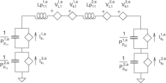
Figure 11.13 PEEC equivalent circuit for electrical surface equation.
Similarly, we also have to take care of the MFIE based on the magnetic current and the field boundary condition in (11.74), or

where ![]() is again the tangential unit vector.
is again the tangential unit vector.
We show the PEEC circuit model corresponding to (11.78) for the magnetic circuit in Fig. 11.14. It is evident that we can choose the same ground node at infinity for both the electric and magnetic interface PEEC model. Further, we did show that the MFIE based in (11.77) is solved by multiplying (11.78) by ![]() . This corresponds to the use of reciprocal medium in the formulation where
. This corresponds to the use of reciprocal medium in the formulation where ![]() is replaced by
is replaced by ![]() and vice versa.
and vice versa.

Figure 11.14 PEEC equivalent circuit for magnetic surface equation.
The surface formulation requires a few observations. First, it is evident from (11.77) that region 1 and region 2 equivalent circuits are connected in series. The inductive surface cells lead to the partial self-inductances for region 1 and the source ![]() is a reminder that the partial mutual inductances are coupled only to cells in region 1 and not region 2. Similarly, the circuit elements for region 2, which are indicated with a superscript 2, restrict the capacitive and inductive couplings to region 2. Finally, the coupled sources
is a reminder that the partial mutual inductances are coupled only to cells in region 1 and not region 2. Similarly, the circuit elements for region 2, which are indicated with a superscript 2, restrict the capacitive and inductive couplings to region 2. Finally, the coupled sources ![]() are restricted to region 1. This can be very helpful for large problems since the coupling is more contained in the regions.
are restricted to region 1. This can be very helpful for large problems since the coupling is more contained in the regions.
The dependent voltage source represents the coupling between the electrical and the magnetic circuits, which is the ![]() terms in (11.77). This leads to an interesting feedback-like coupling situation between the electrical and magnetic circuits.
terms in (11.77). This leads to an interesting feedback-like coupling situation between the electrical and magnetic circuits.
We end the section with a small example that was computed with the PEEC-PMCHWT approach. The geometry is given in Fig. 11.15, which is part of the example given in Ref. [5, 17].
The width of the model is ![]() ,
, ![]() ,
, ![]() , and
, and ![]() and
and ![]() . Here, we chose an example where the number of cells is rather small. This is a more interesting case since important geometries may involve a multitude of such conductors and dielectrics. For both the volume and surface models, the conductors are subdivided using the usual uniform PEEC meshing. The width
. Here, we chose an example where the number of cells is rather small. This is a more interesting case since important geometries may involve a multitude of such conductors and dielectrics. For both the volume and surface models, the conductors are subdivided using the usual uniform PEEC meshing. The width ![]() , thickness
, thickness ![]() , and length
, and length ![]() of conductors are subdivided into 5,2, and 10 divisions, respectively. The dielectric subdivisions are the same for the width and thickness (5 and 2), while the dielectric thickness divisions are chosen to be 5. Figures 11.16 and 11.17 give the imaginary and real parts, respectively, for the current at the terminals of the ac 1 V voltage source. As is apparent, the results compare well.
of conductors are subdivided into 5,2, and 10 divisions, respectively. The dielectric subdivisions are the same for the width and thickness (5 and 2), while the dielectric thickness divisions are chosen to be 5. Figures 11.16 and 11.17 give the imaginary and real parts, respectively, for the current at the terminals of the ac 1 V voltage source. As is apparent, the results compare well.
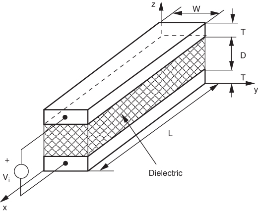
Figure 11.15 Short transmission line model with finite dielectric block.

Figure 11.16 Imaginary part of input current.

Figure 11.17 Real part of input current.
Table 11.2 Run time for volume compared to surface PEEC formulations.
| Subdivision | Volume solution | Volume solution | Surface solution | Surface solution |
| Cell divisions | Number of unknowns | Time (min) | Number of unknowns | Time (min) |
| 4–2–2 | 553 | 0.23 | 756 | 0.61 |
| 6–3–3 | 1348 | 3.7 | 1476 | 3.8 |
| 8–3–4 | 2109 | 14 | 2084 | 10 |
| 10–3–4 | 2997 | 46 | 2488 | 22 |
| 12–4–5 | 4448 | 141 | 3708 | 43 |
For a larger number of cells, the surface formulation takes less computation time. The crossover point from a faster volume cell result to the surface model is shown in Table 11.2. The cell divisions for the dielectric part are given as ![]() –
–![]() for the dielectric in Fig. 11.15. We show that the crossover occurs for 6–3–3 divisions. This is a good comparison since both formulations are using most of the same code and computer. Also, the same implementation of the integrals is used. The exception is the integral for the curl in (11.77) and in (11.77), which are only needed for the surface formulations.
for the dielectric in Fig. 11.15. We show that the crossover occurs for 6–3–3 divisions. This is a good comparison since both formulations are using most of the same code and computer. Also, the same implementation of the integrals is used. The exception is the integral for the curl in (11.77) and in (11.77), which are only needed for the surface formulations.
Problems
- 11.1 Resistance circuit
Use the example of the transformer given in Fig. 11.4 to compute the voltage at each of the three coils in the figure,
 , and
, and  . Assume that the only current is
  . Use the reluctance resistors in (11.20), where each branch has a length of
  , a cross section of
  , and a
  = 850. The number of windings are
  = 15,
= 15,  = 30,
= 30,  . Write a small Matlab program using equations (11.24).
 - 11.2 Inductance computation
For the above problem, compute the
 inductance matrix.
 - 11.3 PEEC formulation
An auxiliary equation in (11.66) is used to include magnetic bodies in PEEC. Verify your understanding of the formula in the third row which represents the magnetic body.
- 11.4 Single-loop inductance
Write a Matlab program to compute the inductance of a square-shaped single loop borrowed from the problems in Chapter 5 of a size of
 with a cross section
  . A magnetic body with
  = 160 is placed at a distance of
  under the loop. The centered magnetic body also of size
  and a thickness of
  is placed under the loop. Compute the inductance of the loop with the magnetic sheet.
 - 11.5 PEEC model for MFIE
Explain each electrical component given in the PEEC circuit model shown in Fig. 11.14 for the magnetic field integral equation (MFIE).
References
- 1. L. V. Bewley. Flux Linkages and Electromagnetic Induction. Dover Publications, New York, 1964.
- 2. J. A. Brandao Faria. Electromagnetic Foundations of Electrical Engineering. John Wiley and Sons, Ltd, Hoboken, NJ, 2nd edition, 2008.
- 3. J. R. Reitz and F. J. Milford. Foundation of Electromagnetic Theory. Pergamon, New York, 1960.
- 4. A. E. Ruehli and D. Ellis. Numerical calculation of magnetic fields in the vicinity of a magnetic body. IBM Journal of Research and Development, 15(6):478–482, November 1971.
- 5. Y. Massoud, J. Wang, and J. White. Accurate inductance extraction with permeable materials using qualocation. Proceedings of the 2nd International Conference of Modeling and Simulation of Micro Structure, Volume 2, Puerto Rico, pp. 151–154, April 1999.
- 6. Y. Yi, V. Sarin, and W. Shi. An efficient inductance extraction algorithm for 3-D interconnects with frequency dependent nonlinear magnetic materials. In Digest of Electrical Performance of Electronic Packaging, San Jose, CA, October 2008.
- 7. W. C. Chew, J.-M. Jin, E. Michielssen, and J. Song. Fast and Efficient Algorithms in Computational Electromagnetics. Artech House, Boston, MA, 2001.
- 8. C. A. Balanis. Advanced Engineering Electromagnetics. John Wiley and Sons, Inc., New York, 1989.
- 9. B. H. Jung, T. K. Sarkar, S. W. Ting, Y. Zhang, Z. Mei, Z. Ji, M. Yuan, A. De, M. Salazar-Palma, and S. M. Rao. Time and Frequency Domain Solutions of EM Problems Using Integral Equations and a Hybrid Methodology. John Wiley and Sons, Inc., New York, 2010.
- 10. K. Umashankar, A. Taflove, and S. Rao. Electromagnetic scattering by arbitrary shaped three-dimensional homogeneous lossy dielectric objects. IEEE Transactions on Antennas and Propagation, 34(6):758–766, June 1996.
- 11. C. A. Balanis. Advanced Engineering Electromagnetics. John Wiley and Sons, Inc., New York, 2012.
- 12. B. M. Kolundzija and A. R. Djordjevic. Electromagnetic Modeling of Composite Metallic and Dielectric Structures. Artech House, Boston, MA, 2002.
- 13. S. M. Rao, C. C. Cha, R. L. Cravey, and D. R. Wilkes. Electromagnetic scattering from arbitrary shaped conducting bodies coated with lossy materials of arbitrary thickness. IEEE Transactions on Antennas and Propagation, 39(5):627–631, May 1991.
- 14. D. Gope, A. Ruehli, and V. Jandhyala. Surface-based PEEC formulation for modeling conductors and dielectrics in time and frequency domain combined circuit electromagnetic simulation. In Digest of Electrical Performance of Electronic Packaging, Volume 13, Portland, OR, pp. 329–332, October 2004.
- 15. A. E. Ruehli, D. Gope, and V. Jandhyala. Mixed volume and surface PEEC modeling. In Proceedings of IEEE Antennas and Propagation Society International Symposium, Volume 11, Monterey, CA, July 2004.
- 16. H. Singer, H.-D. Brüns, and G. Bürger. State of the art in the moment method. In Proceedings of the IEEE International Symposium on Electromagnetic Compatibility, Santa Clara, CA, pp. 122–227, August 1996.
- 17. A. E. Ruehli and G. Antonini. On modeling accuracy of EMI problems using PEEC. In Proceedings of the IEEE International Symposium on Electromagnetic Compatibility, Boston, MA, August 2003.
- 18. Y. Hackl, P. Scholz, W. Ackermann, and T. Weiland. Efficient simulation of magnetic components using the MagPEEC-Method. IEEE Transactions on Magnetics, 53(3), March 2017.