
13
Developing and Deploying PowerPivot Analytics Applications
The end goal of most Business Intelligence projects is to provide data in an easy-to-understand and easy-to-access way for end users to make decisions. No other Business Intelligence tool can fulfill these requirements more than PowerPivot. PowerPivot provides extreme computation power inside a tool that most end users are familiar with and would prefer as their data visualization tool anyway: Excel.
CHOOSING THE RIGHT TOOL FOR THE JOB
PowerPivot can function in two capacities. The first method is PowerPivot for Excel, which is a standalone application. Users can develop high-powered in-memory analytics on their personal machines, which are all self-contained using highly efficient compression algorithms. If users want to share what they have created with others, that leads to the second method, PowerPivot for SharePoint.
PowerPivot for SharePoint allows users to share data models and analysis in a centralized location so the power of the tool is no longer restricted to an end user's desktop. In Lesson 8 you learned how to configure and install PowerPivot for integration with SharePoint 2010 using SQL Server 2008 R2. That lesson set the stage for this one, where you start learning how to develop PowerPivot content and then deploy it to SharePoint.
SQL Server Analysis Services shares many similar features with PowerPivot, but is thought to be a more Enterprise-ready tool, meaning it has additional functionality and scalability features. So the question you must ask yourself before preparing for a project is whether you should use PowerPivot or Analysis Services. For smaller, departmentalized projects PowerPivot is a great solution to provide quick analysis, whereas Analysis Services may take more time to build but it can be easily scaled out to thousands of users.
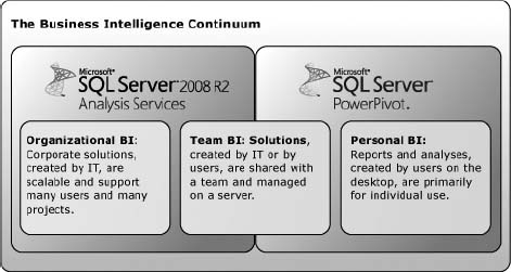
Figure 13-1 describes instances where you may choose one tool over the other. It describes Personal BI as a great example for PowerPivot to shine. A single user, often a business user, develops a PowerPivot report on his or her local desktop and will likely be the sole consumer of it. All that is required for this is a local installation of Microsoft Office Excel 2010 and the PowerPivot add-in.
Organizational BI uses SQL Server Analysis Services and is solely managed by the IT staff. It is an Enterprise-ready solution that can handle major concerns like performance, high availability, and scalability. Organizational BI usually involves much more formal preparation and design processes. This method requires an installation of Analysis Services and Business Intelligence Development Studio.
Team BI refers to the previously described PowerPivot for SharePoint. The reports are designed by either IT staff or business users using Excel. The reports can then be shared and viewed through SharePoint. This technique requires the most set up. You must have Microsoft Office Excel 2010 and the PowerPivot add-in to develop and SharePoint with Analysis Services to manage the PowerPivot workbook data.
DEVELOPING A POWERPIVOT REPORT
Developing PowerPivot Reports is intended to be simple enough for a highly non-technical user to be able to provide significant value. After importing the desired data set into a PowerPivot workbook the user can design a pivot table and chart.
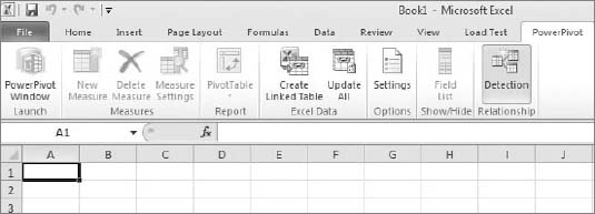
To get started you must install Microsoft Office Excel 2010 and then download and install the PowerPivot for Excel 2010 add-in at www.powerpivot.com. After installing all the necessary components open Excel 2010 and select the new PowerPivot tab in the Office ribbon. Click the PowerPivot Window button to open PowerPivot for Excel, shown in Figure 13-2.
After the PowerPivot window opens you can select from many possible data source connections to import data into PowerPivot. By selecting the From Other Sources button you will see all the data source connections that are available in the native installation. After selecting a connection type you walk through a wizard that will import the data to report on. Figure 13-3 shows the configuration of a connection to SQL Server.

After confirming the connection properties you will be given the option to import the new data either by tables or views from SQL Server, or by query. If you decide to import by query you will be given a query window to write the statement to return the fields that will be used for your pivot table. If you choose to import by object you will be given a list to check off the objects to include. After selecting the objects you want, as shown in Figure 13-4, click Finish.
When you click Finish you will be able to see the objects being imported. When this completes, click Close to return to the PowerPivot window. Database relationships are carried over to PowerPivot, but if you need to make changes you can do this on the Design tab with the Manage Relationships button. Now that the data is imported you can create a report by clicking the PivotTable button on the Office ribbon. This returns you to Excel where you will be given the option to create a new worksheet or use an existing one for your report.
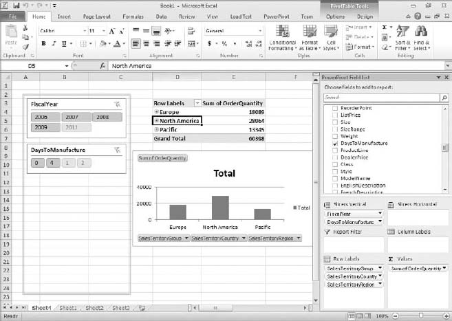
Next, use the PowerPivot Field List to select the fields that you want to display in your report. The items that are selected from this list are automatically added to the report in a PivotTable, PivotChart, or Slicers. Slicers are a new data visualization tool to Excel 2010 that allows the user to better see which records the report is being filtered on. Figure 13-5 shows the PowerPivot Field List and a completed report that uses a PivotTable, PivotChart, and Slicers.

INTRODUCTION TO DATA ANALYSIS EXPRESSIONS (DAX)
Data Analysis Expressions (DAX) is what you will use to extend the capabilities of PowerPivot. DAX is similar to the Excel formula language, making it easier for current Excel users to learn. The newly provided DAX functions bring many of the SQL Server Analysis Service concepts to PowerPivot. For example, you can use the DAX function DATESYTD to calculate year-to-date figures of a measure.
You can write DAX functions in two places. The first place is in the PowerPivot window by using a Calculated Column. Calculated Columns are a way that you can add additional fields for the purposes of displaying in a report, creating relationships where they did not exist previously, or returning some quick analysis of the data. This would be comparable to a derived column in SQL Server. Figure 13-6 shows that Calculated Columns are written in the same place as typical Excel formulas. After scrolling to the farthest right point of the document you will see Add Column. Select this column and you will be able to write your expression and rename the column.

The Calculated Column Example shown in the following table provides many common DAX expressions used as Calculated Columns.
The second place DAX functions can be used is in Calculated Measures. These expressions are written not in the PowerPivot window, but instead in the PowerPivot Field List of a report. This would be comparable to an MDX calculation in Analysis Services.
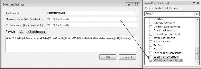
To create a Calculated Measure, under the Home tab in the PowerPivot window select the PivotTable button and then PivotTable again from the drop-down box. Click OK when the Create PivotTable dialog box opens inside of Excel. Next, right-click in the PowerPivot Field List on the table in which you would like to create a Calculated Measure and select Add New Measure. In the Measure Settings dialog box name the measure and write the DAX formula shown in Figure 13-7 to complete the calculation.
The Calculated Column Example shown in the following table provides many common DAX expressions used as Calculated Measures.
CREATING AND DEPLOYING REPORTS TO A POWERPIVOT GALLERY
The PowerPivot Gallery is a SharePoint document library that can graphically preview each report to your end users before actually selecting them. In Lesson 8 you learned how to install and configure PowerPivot for SharePoint. If you have a standalone server install of PowerPivot for SharePoint, a PowerPivot Gallery is created for you upon the completion of the install. If the install was done to an existing SharePoint farm, you must create a PowerPivot Gallery manually. You can choose either to create a new PowerPivot site that includes a PowerPivot Gallery library or add the PowerPivot Gallery library to an existing site.
To create the PowerPivot site open your web browser and enter the URL http://<YourServerName> where SharePoint has been installed. Select the Site Actions drop-down box in the top left of the page and click New Site. Figure 13-8 shows the available template sites, from which you will select PowerPivot Site. Give the site a title and URL name and click Create. This site will automatically provide you with a PowerPivot Gallery so there is no need to manually add it.

If you simply need to add the PowerPivot Gallery as a library to an existing site, select Site Actions in the top left of the page and click View All Site Content. After the All Site Content page opens click the Create button to create a new library. Figure 13-9 shows that by using the Library filter you can easily find the PowerPivot Gallery. Select the PowerPivot Gallery, give it a name, and click Create.

Now that you have a PowerPivot Gallery available for deployment open a PowerPivot workbook in Excel 2010. After the workbook you want to deploy opens click the File tab. Click Save & Send and select Save to SharePoint. Click Browse for a Location, which opens the Save As dialog box. In the file path box type http://<YourServerName> to connect to your SharePoint instance as shown in Figure 13-10. Open the PowerPivot Gallery and click Save. Before saving you can optionally click the Publish Options button to select which Excel sheets are deployed; by default the entire workbook is deployed, including blank sheets.
Once it has completed the deployment it will automatically open the document from SharePoint. If you would like to view all the documents in the PowerPivot Gallery navigate to the path where you just completed your deployment. By default the documents are shown in the Gallery view, but you can optionally change it to the popular Carousel view by clicking the Library tab at the top of the page and then selecting Carousel from the Current View drop-down box, as shown in Figure 13-11.


TRY IT
In this Try It you combine the three main topics of this lesson to complete your task. You first develop a basic PowerPivot report and then create a Calculated Measure using DAX. Finally, you deploy the result to a PowerPivot Gallery.
Lesson Requirements
To complete this lesson you need to have SharePoint 2010 already installed. If you have not done this yet, please refer to Lesson 8, which walks you through the installation steps. You must also have Excel 2010 with the PowerPivot add-in installed. The step-by-step example uses the AdventureWorks sample databases, which you can download from www.codeplex.com.
Hints
- Develop a PowerPivot workbook that uses the FactResellerSales table from the AdventureWorksDW2008R2 database. You should also select the related tables of FactResellerSales.
- Create a Calculated Measure on FactResellerSales that will allow you to do a comparison between the current SalesAmount column and the SalesAmount from the same period but from the previous year.
- Build a report that displays SalesAmount and the newly created measure.
- Create a PowerPivot site in SharePoint and deploy your report to the PowerPivot Gallery.
Step-by-Step
- Go to Start
 All Programs Microsoft Office Microsoft Excel 2010.
 - After Excel opens select the PowerPivot tab in the Office ribbon and click PowerPivot Window to launch PowerPivot for Excel.
- Click the From Database drop-down box and select From SQL Server.
- In the Connect to a Microsoft SQL Server Database dialog box enter the server name property of the server on which you installed the AdventureWorks sample. Select AdventureWorksDW2008R2 from the Database Name drop-down box and click Next.
- In the Choose How to Import the Data dialog box leave the default setting of “Select from a list of tables and views to choose the data to import” and click Next.
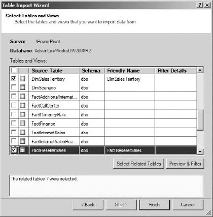
- Select the FactResellerSales table and click the Select Related Tables button. Figure 13-12 shows you should have a total of seven tables selected. Click Finish.
- The wizard next imports all the data into PowerPivot. When this completes, click Close.
- Each table is now imported into PowerPivot for Excel. To create a report click the PivotTable drop-down box on the Home tab and select Chart and Table (Horizontal). This returns you to Excel to create the report.
- Click OK to create the PivotChart and PivotTable in a new worksheet.
- In the PowerPivot Field List right-click the FactResellerSales table and click Add New Measure.
- Name the measure PriorYearSalesAmount and type the following formula as shown in Figure 13-13:
=CALCULATE(SUM(FactResellerSales[SalesAmount]),DATEADD(DimDate[FullDateAlternateKey],−1,YEAR),All(DimDate))
- Verify the formula works by clicking the Check Formula button and click OK. After, the measure will automatically be added to the report.
- The chart and table work independently from each other so select the object that did not get PriorYearSalesAmount automatically added to it, then check it in the PowerPivotFieldList to add it there as well. You may need to click Refresh in the field list to get the field added.
- Add SalesAmount from FactResellerSales to the Values box of both the chart and table.
- From the DimDate table select CalendarYear to be added to the Axis Fields of the chart and the Row Labels of the table.
- From the DimSalesTerritory table add the SalesTerritoryCountry field to the Slicers Horizontal section. Your report and PowerPivot Field List selections should look similar to Figure 13-14.

- The last step is to deploy the report to a PowerPivot Gallery. Open a web browser and type in your SharePoint server: http://<YourServerName>.
- Select Site Actions in the top left of the page and click New Site.
- Choose the PowerPivot Site template and give it a title of Lesson13. Make the URL name also Lesson13 and click Create.
- Now that the PowerPivot site is created return to Excel to deploy the document to the PowerPivot Gallery.
- Inside Excel select the File tab and choose Save & Send.
- Click Save to SharePoint and select Browse for a Location. This opens the dialog box to save your document.
- In the file path box type in your SharePoint server name: http://<YourServerName>.
- Navigate to the Lesson13 PowerPivot site that was just created and open the PowerPivot Gallery document library.
- Change the File Name to Lesson13CompletedStepByStep and click Save.
- Once the deployment has completed the document will automatically be opened in SharePoint. Navigate to the Lesson13 PowerPivot site in your web browser and open the PowerPivot Gallery to view the reports. The PowerPivot Gallery should look like Figure 13-15.


Congratulations! You have just created a PowerPivot report and deployed it to a PowerPivot Gallery in SharePoint.
 Please select Lesson 13 on the DVD to view the video that accompanies this lesson.